
#50=,9:0;@6-,5;<*2@#50=,9:0;@6-,5;<*2@
#56>3,+.,#56>3,+.,
"/,:,:(5+0::,9;(;065:.90*<3;<9(3
*65640*:
#56>3,+.,
" !!&!"" " !!&!""
"!!"!!
)+,3(A0A(>(50
#50=,9:0;@6-,5;<*2@
()+,3(>(50<2@,+<
0.0;(3)1,*;+,5;0C,9/;;7:+6069.,;+
0./;*30*2;667,5(-,,+)(*2-69405(5,>;();63,;<:256>/6>;/0:+6*<4,5;),5,C;:@6< 0./;*30*2;667,5(-,,+)(*2-69405(5,>;();63,;<:256>/6>;/0:+6*<4,5;),5,C;:@6<
,*644,5+,+0;(;065 ,*644,5+,+0;(;065
(>(50)+,3(A0A" !!&!"" "!
!
"/,:,:(5+0::,9;(;065:.90*<3;<9(3*65640*:
/;;7:<256>3,+.,<2@,+<(.,*65',;+:
"/0:6*;69(30::,9;(;0650:)96<./;;6@6<-69-9,,(5+67,5(**,::)@;/,#56>3,+.,(;#56>3,+.,;/(:
),,5(**,7;,+-6905*3<:06505"/,:,:(5+0::,9;(;065:.90*<3;<9(3*65640*:)@(5(<;/690A,+(+4050:;9(;696-
#56>3,+.,69469,05-694(;06573,(:,*65;(*;#56>3,+.,3:=<2@,+<
!"#" "!"#" "
9,79,:,5;;/(;4@;/,:0:69+0::,9;(;065(5+():;9(*;(9,4@690.05(3>692967,9(;;90)<;065
/(:),,5.0=,5;6(336<;:0+,:6<9*,:<5+,9:;(5+;/(;(4:63,3@9,:765:0)3,-696);(0505.
(5@5,,+,+*67@90./;7,940::065:/(=,6);(05,+5,,+,+>90;;,57,940::065:;(;,4,5;:
-964;/,6>5,9:6-,(*/;/09+7(9;@*67@90./;,+4(;;,9;6),05*3<+,+054@>692(336>05.
,3,*;9650*+0:;90)<;0650-:<*/<:,0:56;7,940;;,+)@;/,-(09<:,+6*;905,>/0*/>033),
:<)40;;,+;6#56>3,+.,(:++0;065(303,
/,9,)@.9(5;;6"/,#50=,9:0;@6-,5;<*2@(5+0;:(.,5;:;/,099,=6*()3,565,?*3<:0=,(5+
96@(3;@-9,,30*,5:,;6(9*/0=,(5+4(2,(**,::0)3,4@>69205>/63,69057(9;05(33-694:6-
4,+0(56>69/,9,(-;,9256>5(.9,,;/(;;/,+6*<4,5;4,5;065,+()6=,4(@),4(+,
(=(03()3,044,+0(;,3@-69>693+>0+,(**,::<53,::(5,4)(9.6(7730,:
9,;(05(336;/,96>5,9:/0790./;:;6;/,*67@90./;6-4@>692(3:69,;(05;/,90./;;6<:,05
-<;<9,>692::<*/(:(9;0*3,:69)662:(33697(9;6-4@>692<5+,9:;(5+;/(;(4-9,,;6
9,.0:;,9;/,*67@90./;;64@>692
$% $" $% $"
"/,+6*<4,5;4,5;065,+()6=,/(:),,59,=0,>,+(5+(**,7;,+)@;/,:;<+,5;B:(+=0:6965
),/(3-6-;/,(+=0:69@*6440;;,,(5+)@;/,09,*;696-9(+<(;,!;<+0,:!65),/(3-6-
;/,796.9(4>,=,90-@;/(;;/0:0:;/,C5(3(7796=,+=,9:0656-;/,:;<+,5;B:;/,:0:05*3<+05.(33
*/(5.,:9,8<09,+)@;/,(+=0:69@*6440;;,,"/,<5+,9:0.5,+(.9,,;6()0+,)@;/,:;(;,4,5;:
()6=,
)+,3(A0A(>(50!;<+,5;
90*/(,3 ,,+(16996-,::69
9(93 0336509,*;696-9(+<(;,!;<+0,:

THREE ESSAYS ON THE APPLICATION OF MACHINE LEARNING METHODS
IN ECONOMICS
DISSERTATION
A dissertation submitted in partial fulfillment of the
requirements for the degree of Doctor of Philosophy in the
College of Agriculture, Food and Environment
at the University of Kentucky
By
Abdelaziz Lawani
Lexington, Kentucky
Co-Directors: Dr. Michael Reed, Professor of
International Trade and Agricultural Marketing
and Dr. Yuqing Zheng, Associate Professor of
Food Marketing and Policy Analysis
Lexington, Kentucky
2018
Copyright © Abdelaziz Lawani 2018
ABSTRACT OF DISSERTATION
THREE ESSAYS ON THE APPLICATION OF MACHINE LEARNING METHODS
IN ECONOMICS
Over the last decades, economics as a field has experienced a profound transformation
from theoretical work toward an emphasis on empirical research (Hamermesh, 2013).
One common constraint of empirical studies is the access to data, the quality of the data
and the time span it covers. In general, applied studies rely on surveys, administrative or
private sector data. These data are limited and rarely have universal or near universal
population coverage. The growth of the internet has made available a vast amount of
digital information. These big digital data are generated through social networks, sensors,
and online platforms. These data account for an increasing part of the economic activity
yet for economists, the availability of these big data also raises many new challenges re-
lated to the techniques needed to collect, manage, and derive knowledge from them.
The data are in general unstructured, complex, voluminous and the traditional software
used for economic research are not always effective in dealing with these types of data.
Machine learning is a branch of computer science that uses statistics to deal with big data.
The objective of this dissertation is to reconcile machine learning and economics. It uses
threes case studies to demonstrate how data freely available online can be harvested and
used in economics. The dissertation uses web scraping to collect large volume of unstruc-
tured data online. It uses machine learning methods to derive information from the un-
structured data and show how this information can be used to answer economic questions
or address econometric issues.
The first essay shows how machine learning can be used to derive sentiments from re-
views and using the sentiments as a measure for quality it examines an old economic the-
ory: Price competition in oligopolistic markets. The essay confirms the economic theory
that agents compete for price. It also confirms that the quality measure derived from sen-
timent analysis of the reviews is a valid proxy for quality and influences price. The sec-
ond essay uses a random forest algorithm to show that reviews can be harnessed to pre-

dict consumers’ preferences. The third essay shows how properties description can be
used to address an old but still actual problem in hedonic pricing models: the Omitted
Variable Bias. Using the Least Absolute Shrinkage and Selection Operator (LASSO) it
shows that pricing errors in hedonic models can be reduced by including the description
of the properties in the models.
KEYWORDS: Machine Learning, Hedonic Price Model, Sentiment Analysis, Random
Forest, Omitted Variable Bias, LASSO
Abdelaziz Lawani
July 22
nd
, 2018

THREE ESSAYS ON THE APPLICATION OF MACHINE LEARNING METHODS
IN ECONOMICS
by
Abdelaziz Lawani
Prof. Michael Reed
Co-Director of Dissertation
Dr. Yuqing Zheng
Co-Director of Dissertation
Prof. Carl R. Dillon
Director of Graduate Studies
July 22
nd
, 2018
Anna-Liisa, T’del Karl, Marie-Madeleine, and Nathalia Nakaambo, this work is dedicat-
ed to you. When I embarked in this journey a few years ago, little did I know that it was
going to be not only intellectual but also emotional and spiritual. We learned, overcame
challenges, and grew together. You are the real Ph.Ds.!
iii
ACKNOWLEDGMENTS
The completion of this dissertation would not have been possible without the guidance
and advice of my advisors Prof. Reed Michael and Dr. Yuqing Zheng. I remember their
reactions when I first presented my idea to them a few years ago. It was a mix of curiosi-
ty, excitement, and encouragement. They offered me the freedom necessary to unleash
my intellectual curiosity, dig into challenging questions, gain the knowledge and skills
from other fields, and develop the confidence needed to address the questions subject of
this dissertation. Their suggestions and insightful comments have been crucial in turning
a raw idea into a polished topic.
I would extend my sincere appreciation to Prof. Leigh Maynard who arduously supported
me in expanding my passion for research for development and entrepreneurship. He
helped me look beyond the academia and use my knowledge and skills to address some
of the world most pressing challenges.
I also want to thank the staff, students, and faculty members of the Department of Agri-
cultural Economics at the University of Kentucky. It was comforting to see the familial
atmosphere in the department and their efforts to give the students the best education pos-
sible. Their support played a significant role in my success. I remember the words of en-
couragement of Rita, and Karen and the extraordinary efforts of Kristen helping me get
the materials needed for my works.
Finally, this dissertation would not have been possible without the support from my fami-
ly. My wife Anna-Liisa Ihuhwa was my rock. She provided me with the mental stamina
during the whole process. The process will also see the birth of our son T’del Karl. He
brought us joy and happiness, and his first steps are the inspiration behind this disserta-
tion. I saw him fall and crawl so many times, yet he never fails to always try one more
time. This mental image was my inspiration. The process would not be complete without
my family members in Benin and Namibia. I never felt alone during the journey because
you were always there.
TABLE OF CONTENTS
Acknowledgments.............................................................................................................. iii
Table of Contents ............................................................................................................... iv
List of Tables .................................................................................................................... vii
List of figures ................................................................................................................... viii
Chapter 1 : General introduction......................................................................................... 1
Chapter 2 : Impact of reviews on price: Evidence from sentiment analysis of Airbnb
reviews in Boston ................................................................................................................ 4
2.1. Abstract .................................................................................................................... 4
2.2. Introduction .............................................................................................................. 4
2.3. Literature review ...................................................................................................... 7
2.4. Conceptual framework ........................................................................................... 10
2.5. Data and Methods ................................................................................................... 15
2.5.1. Data ................................................................................................................. 15
2.5.2. Derivation of quality scores with sentiment analysis of the reviews .............. 18
2.6. Econometric results and discussion ........................................................................ 25
2.7. Sensitivity analysis ................................................................................................. 31
2.8. Conclusion .............................................................................................................. 38
Chapter 3 Chapter 3. Text-based predictions of beer preferences by mining online
reviews .............................................................................................................................. 40
3.1. Abstract: ................................................................................................................. 40
3.2. Introduction ............................................................................................................ 40
3.3. Literature review .................................................................................................... 43
3.4. Methodology .......................................................................................................... 47
3.4.1. Feature extraction ............................................................................................ 48
3.4.2. Feature selection ............................................................................................. 49
3.4.3. Predictive model: the random forest ............................................................... 51
v
3.5. Results and discussions .......................................................................................... 57
3.5.1. N-grams representation ................................................................................... 57
3.5.2. Term frequency vs inverse document frequency ............................................ 59
3.5.3. Performance analysis of the random forest classifier for the unigram-inv
model......................................................................................................................... 60
3.5.4. Effect of number of trees on the model accuracy ........................................... 62
3.5.5. Identification of the most important features in the reviews .......................... 63
3.6. Conclusion .............................................................................................................. 66
Chapter 4 : Textual analysis and omitted variable bias in hedonic price models applied to
short-term apartment rental market. .................................................................................. 68
4.1. Abstract .................................................................................................................. 68
4.2. Introduction ............................................................................................................ 68
4.3. Data and estimation procedure ............................................................................... 71
4.3.1. Data ................................................................................................................. 71
4.3.2. Estimation procedure ...................................................................................... 74
4.3.3. Unigram representation of the description of rental rooms ............................ 74
4.3.4. Penalized regression: The Least Absolute Shrinkage and Selection Operator
(LASSO) ................................................................................................................... 77
4.4. Results and discussion ............................................................................................ 79
4.4.1. Comparison of the regression models ............................................................. 79
4.4.2. LASSO estimates of the BOW-time-location fixed effects hedonic pricing
model......................................................................................................................... 82
4.4.3. Pricing value of the features. .......................................................................... 84
4.5. Conclusion .............................................................................................................. 87
Chapter 5 : General conclusion ......................................................................................... 89
Glossary ............................................................................................................................ 91
References ......................................................................................................................... 94
vi
Vita .................................................................................................................................. 106
vii
LIST OF TABLES
Table 2.1: Description and summary statistics of the variables ........................................ 17
Table 2.2: Sample of reviews and their score ................................................................... 20
Table 2.3: Moran I test ...................................................................................................... 22
Table 2.4: OLS regression diagnostic test for spatial dependence ................................... 22
Table 2.5: Estimates of the spatial lag regressions with 1 mile as weight matrix ............ 26
Table 2.6: Direct, indirect and total effects of the impact of the regressors on room price
........................................................................................................................................... 27
Table 2.7: Decomposition of the impact of review score for flexible, moderate, strict and
super strict cancellation policies ....................................................................................... 30
Table 2.8: Likelihood ratio tests for the statistical significance of price lag and quality
variables in the linear mixed effects models ..................................................................... 32
Table 2.9: Estimates of the spatial lag regression with 3 and 5 miles as weight matrix ... 34
Table 2.10: Impact of alternative measures of quality on price ........................................ 36
Table 2.11: Decomposition estimates of the direct and indirect effects of quality variables
on rooms' prices ................................................................................................................ 36
Table 3.1: Number of features selected with the Boruta algorithm .................................. 51
Table 3.2: Models accuracy and Kappa statistic ............................................................... 58
Table 3.3: Confusion matrix of the unigram-inverse random forest model ..................... 60
Table 4.1: Description and summary statistics for Airbnb data in San Francisco ............ 72
Table 4.2: Sample of description of the rental units on Airbnb in San Francisco ............ 73
viii
LIST OF FIGURES
Figure 2.1: Frequency of the languages used to write the reviews on Airbnb in Boston . 21
Figure 2.2: Boxplot of price by cancellation policy ......................................................... 29
Figure 3.1: Performance comparison of the unigram, bigram, trigram models and their
inverse ............................................................................................................................... 58
Figure 3.2: Receiver Operator Curve (ROC) and Area Under the Curve (AUC) for the
unigram-inverse random forest model .............................................................................. 62
Figure 3.3: Effect of the number of trees on Out of Bag, Good, and "Very Good"
categories error rate estimates ........................................................................................... 63
Figure 3.4: Importance of the features in the unigram inverse predictive random forest
model................................................................................................................................. 65
Figure 4.1: Word cloud representation of the rental unit description on Airbnb in San
Francisco ........................................................................................................................... 76
Figure 4.2: Number of features selected by the LASSO model as function of the Lambda
parameter ........................................................................................................................... 83
Figure 4.3: Cross-validated mean estimates of the MSE as a function of the Lambda
parameter ........................................................................................................................... 84
Figure 4.4: Estimates of the most important significant positive and negative variables . 85
1
CHAPTER 1 : GENERAL INTRODUCTION
Other the last two decades, the web 2.0 has reshaped the structures and conditions
of diverse markets such as transportation, travel, books, banking, energy, and healthcare.
Contrary to the first generation of static web pages on the internet, the web 2.0 refers to
dynamic pages such as social media or online platforms where the users can interact.
Online platforms such as Amazon, Netflix, eBay, Alibaba, Uber, LinkedIn, Zipcar, and
Airbnb are now household names. They create value by facilitating the transaction of
products and services between two or more economic agents who would otherwise have
difficulty finding each other (Evans et al. 2011). Online platforms offer the possibilities
for different agents to interact and record the nature and content of the billions of interac-
tions and transactions that occur on the platforms. They are disrupting major industries,
and the volume of transactions on these platforms is consistently increasing. According to
the U.S. Census Bureau (2017), online sales accounted for 8.2 percent of total sales in the
second quarter of 2017 and rose by 16.3 percent compared to the second quarter of 2016;
total retail sales increased by only 4.4 percent during the same period. As the volume of
transactions for online platforms increases, so do the number of people using these plat-
forms and the size of data generated by the platforms. However, applied research on plat-
forms in the economics literature has not followed the same growth.
The development of online platforms has made available a considerable volume of data.
Social networks, geo-location, impressions through tweets, online purchases, and mobile
phone data, are a few examples of data sources that can allow novel research in social
science. For economists, the availability of this amount of data is an opportunity to ob-
2
serve consumers’ revealed preferences through their behavior online. These data can also
address some econometrics issues (e.g., omitted variable bias and instrumental variables)
faced when estimating causal relationships in non-experimental designs. The availability
of these big data also raises many new challenges related to the techniques needed to col-
lect, manage, and derive knowledge from them. These challenges can be overcome by
borrowing the techniques and skills needed to deal with big data from other disciplines
such as statistics and computer science. Machine learning combines computer science
and statistics to handle and derive relevant information from big data, and the present dis-
sertation offers three essays on the application of machine learning methods in econom-
ics.
The first essay examines the relationship between guests reviews, used as a proxy for
quality, and the price set by hosts on the Airbnb platform in Boston. Using sentiment
analysis to derive the quality from the reviews and a hedonic spatial autoregressive model
applied to rental room prices on Airbnb, the finding of this essay suggest that prices are
strategic complements and are influenced by the review score, the characteristics of the
room, and the features of the neighborhood. The marketing implication is that consumers
respond to the contents of online reviews, in addition to customer ratings. The results of
this essay show that policies that improve the quality of the room for one host will have a
spillover effect on the price of rooms offered by other hosts.
The second essay uses text categorization and random forest to predict beer preferences.
It compares six text categorization procedures: frequency terms of unigrams, bigrams,
trigrams, and their inverse frequency terms. With data scrapped from BeerAdvocate, an
online network of independent consumers and professionals in the beer industry, this es-
3
say shows that the words used in the reviews can predict consumer’s preferences. Moreo-
ver, it indicates that the use of less frequent terms in the predictive models outperforms
the use of more frequent terms, confirming Sparck Jones (1972)’s heuristics results.
However, low-level combinations of the words in the reviews better predict consumers’
preferences compared to high-level combinations, even though the latter better represent
the complexity of human languages.
The third essay addresses the omitted variable bias problem in hedonic pricing models
using unigram text categorization. The presence of omitted variables is a source of bias
for the estimates of hedonic models. The solutions adopted in the real estate literature
have struggled to deal effectively with this issue. This essay uses textual analysis to ad-
dress the omitted variable bias problem. It explores a method of proxying the variables
omitted in the hedonic regression models with the words used in the description of the
rental units. The results show that this solution reduces the pricing error in the hedonic
models and can be useful in accounting for omitted quality measures in hedonic price
models.
4
CHAPTER 2 : IMPACT OF REVIEWS ON PRICE: EVIDENCE FROM
SENTIMENT ANALYSIS OF AIRBNB REVIEWS IN BOSTON
2.1. Abstract
There is a growing interest in deriving value from user-generated comments and reviews
online. For businesses and consumers using online platforms, the reviews serve as quality
metrics and influence consumers purchasing decision. This study examines the
relationship between guests reviews, used as a proxy for quality, and the price set by
hosts on the Airbnb platform in Boston. Using sentiment analysis to derive the quality
from the reviews and a hedonic spatial autoregressive model applied to rental room prices
on Airbnb, we find that prices are strategic complements and are influenced by the
review score, the characteristics of the room, and the features of the neighborhood. The
marketing implication is that consumers respond to the contents of online reviews, in
addition to customer ratings. Policies that improve the quality of the room for one host
will have a spillover effect on the price of rooms offered by other hosts.
2.2. Introduction
Many platforms allow customers to write a review for the sellers they use or for
the products (or services) they purchase (e.g., eBay, Amazon, Priceline). This allows po-
tential consumers to go through multiple reviews about products or services before mak-
ing their purchasing decisions. They use the opinions in the reviews to form their own
opinion about the quality of the product or service they want to purchase. Reviews are
becoming even more important for experience goods such as hotel rooms and rental
houses, which are purchased at distance (Viglia, et al., 2016) with the quality being hard
for travelers to assess before consumption (Klein, 1998).
5
Researchers have shown increasing interests in understanding the opinions and
feelings hidden in the millions of reviews left by consumers online (Liu, et al., 2005,
Pang and Lee, 2008). Reviews, scored or rated in terms of satisfaction by customers, in-
fluence purchase probability of online shoppers (Kim and Srivastava, 2007). Different
schemes of rating are used on online platforms. They commonly vary from bimodal,
thumbs up or thumbs down, to scale from one to five stars (Sarvabhotla, et al., 2010).
According to Archak, et al. (2011), numerical or bimodal ratings do not accurately cap-
ture the information embedded in the reviews and may not express precise details to pro-
spective shoppers. Using predictive modeling, they show the effect of different product
features in the reviews on sales, confirming the importance of the words used in the
reviews to evaluate the products. Chevalier and Mayzlin (2006) show that customers rely
more on the reviews than the rating scores.
In the hotel industry literature, the presence of consumer reviews and ratings are
found to drive sales (Blal and Sturman, 2014, Floyd, et al., 2014, Ye, et al., 2009). Most
of the studies use star ratings and customer ratings as a proxy for the quality in the re-
views but not the words in the reviews. Yet, there is no agreement on i) the relationship
between hotel reviews and quality, and ii) the impact of reviews on price. For examples,
Öğüt and Onur Taş (2012), using star ratings and customer ratings, find that these quality
metrics increase hotels price and online sales. Contrary, a recent study by Viglia, et al.
(2016), finds a positive association between review scores and hotel occupancy rates, but
not a significant relationship between reviews and star ratings, suggesting that these two
measures involve two different concepts of quality, contrary to the existing literature on
reviews and quality.
6
The present study contributes to the online marketing literature on the relationship
between guests’ reviews and quality, and their impact on price. Unlike previous research
that uses review score such as the number of reviews, star rating and customer rating, this
study derives the constructs of quality from the opinions in the reviews with sentiment
analysis. Sentiment analysis is a methodology, often used in computer science, to extract
value, opinions or attitudes toward products or services from reviews (Bautin, et al.,
2008, Hu and Liu, 2004, Pang and Lee, 2008, Ye, et al., 2009). Using data collected from
Airbnb in Boston and a spatial autoregressive hedonic model, the analysis shows that the
price of a room on the platform depends not only on the intrinsic characteristics of the
room and its location, but also on the price set by other hosts in the neighborhood. The
price of a room is also correlated with the quality score derived from sentiment analysis
of its reviews. The spatial nature of the estimation method implies that the quality
measure, derived from the reviews of a room, has not only a direct effect on the room
price but also a spillover effect on the price of rooms in its neighborhood.
The remainder of this paper is organized as follows. In section 2 we give an
overview of the relevant literature. Section 3 presents the conceptual framework. Section
4 introduces the data and the spatial autoregressive estimation method, including a
detailed description of the sentiment analysis methodology. Results of the spatial hedonic
pricing model are presented in section 5. Finally, section 6 concludes.
7
2.3. Literature review
The importance of word-of-mouth (WOM) on consumer purchasing decision has
been widely examined in the economic literature (Brooks, 1957, Kozinets, et al., 2010,
Liu, 2006). WOM contents are user-generated comments, reviews, ratings, and other
communications and are perceived to be more credible than advertising (Mauri and
Minazzi, 2013, Ogden, 2001) since they are real user experiences and not paid ads.
Litvin, et al. (2008) stresses the importance of the independence of the source of the mes-
sage for WOM to be considered as a reliable source of information by customers. This is
well illustrated by Mauri and Minazzi (2013) experimental study where hotel guests re-
views are positively correlated with customers’ hotel purchasing intention, but the pres-
ence of hotel managers’ responses to the guest's reviews leads to a negative correlation
with their purchasing intention. Zhang, et al. (2010) confirm this finding. Using data col-
lected from Dianping.com on restaurants, they compare the popularity of consumers’ re-
views with professional editors’ reviews. Their study shows that consumers-created re-
views are more popular than editors’ reviews, as indicated by the number of page views.
There is a substantial number of studies in economics on the effect of reviews on
sales. De Vany and Walls (1999), Dellarocas, et al. (2007) and Liu (2006) show the im-
pact of reviews on box office revenue. In the service industry, reviews are considered as a
primary source of information on quality (Hu, et al., 2008) as they reduce information
asymmetry, and allow consumers to have better information about the attributes of the
service they want to purchase (Nicolau and Sellers, 2010). Luca (2016), studying the im-
pact of reviews and reputation on restaurant revenue in Washington, finds that a one-star
increase in Yelp’s rating increases a restaurant’s revenue by 5-9 percent. Zhang, et al.
8
(2013), studying the determinants of camera sales, finds that the average online customer
review, as well as the number of reviews, are significant predictors of digital camera
sales.
In the hotel industry, reviews affect hotel room purchase intention, sales, and
price. According to O’Connor (2008), increasing numbers of travelers consult feedback
left by other customers while planning their trip. Gretzel and Yoo (2008) estimate that
75% of travelers use the feedback of other consumers whilst making travel arrangements.
Vermeulen and Seegers (2009), through an experimental study in the Netherlands, con-
firm that online reviews affect consumers’ choice in the hotel industry, but this effect is
asymmetric. Results from their study indicate that positive and negative reviews do not
have the same impact on a consumer’s behavior. Positive reviews have a positive impact,
but negative reviews have a smaller impact in absolute value than positive reviews. With
regard to sales and price, Ye, et al. (2011), exploiting data from a major travel agency in
China, show that a 10 percent increase in traveler rating increases the volume of online
reservations by more than 5 percent. Öğüt and Onur Taş (2012) also find that more posi-
tive online customer ratings increase hotel room prices and online sales.
Quality has many dimensions and measures and customer ratings might only cap-
ture a small part of it. During the rating process, customers may refer not only to the
quality of the product or service but also to its price, or both. Even when referring to the
quality, some features of the product or service are considered more important than oth-
ers, depending on the taste of the customer. Zhang, et al. (2011) show a heterogeneous
impact of rating on hotel room prices. They found the impact to be only noticeable for
economy and midscale hotels and not for luxury hotels where location and the quality of
9
services are the most important factors that determine consumers’ willingness to pay.
They use different ratings such as cleanliness, quality of room, location, and service and
found different impacts of these ratings on price. The findings of Li and Hitt (2010) con-
firms the results of Zhang, et al. (2011). According to Li and Hitt (2010) both quality and
price influence purchase decision. Their empirical analysis on digital cameras shows that
ratings, being in general unidimensional, are biased by prices and are more closely corre-
lated with the product value than its quality. More recently, Viglia, et al. (2016) find a
positive association between review score and hotel occupancy rate. They use diverse
categories of hotels and various online review platforms and find that a one point increase
in the review score increases the hotel occupancy rate by 7.5 percentage points. However,
they did not find any association between review score and star rating. For Viglia, et al.
(2016) review score and star rating might reflect different measures of quality.
There is a need to clarify the relationship between reviews and price. Most of the
studies on the impact of reviews on price and sales in the hotel industry literature use
rating or single review scores that might not represent the complexity of the customer
opinion or sentiment about a good or service accurately. Allowing for a methodology,
such as sentiment analysis, that mines the client's opinion in the reviews is more likely to
depict correctly the quality of the good or service he/she receives. Using sentiment
analysis, this study examines the role of opinions derived from reviews in consumer
valuation and prices. It uses data collected in the short-term apartment rental market on
Airbnb in Boston. The sentiment expressed by the reviews on the platform serves as an
intrinsic indicator of the quality of the service offered by the hosts. The indicator is then
used to empirically test if reviews affect price and if multidimensional ratings have
10
identical effects on price. Our contribution is twofold. First, we use sentiment analysis to
examine how the contents of online reviews could affect prices, rather than relying on
customer ratings. Second, with a unique dataset, we test whether rental rooms’ prices are
spatially correlated, and if so, whether rental prices are strategic complements or
substitutes.
2.4. Conceptual framework
An interesting feature of online platforms, such as Airbnb, is the possibility for
both hosts and guests to learn about each other before accepting the transaction. By facili-
tating direct interaction between participants on two sides, these platforms offer partici-
pants the possibility to control the terms of their interaction; the intermediary does not
take control of these terms (Hagiu and Wright, 2015). On the Airbnb platform, hosts de-
cide on the bundle of services they will offer (bed, couch or sofa, shared bed, Wi-Fi, etc.)
and the price of their service. Guests have the possibility to define the nature and quality
of the services they desire. For hosts, this has direct implications on their competitive-
ness. The quality of reviews left by guests can impact their business positively (if the
review is positive) or negatively (if the review is negative). Hosts can also learn from
their competitors and adjust their price and quality accordingly. This type of interaction
where participants on one side of the network compete is referred to as inside competition
or a same-side negative effect (Eisenmann, et al., 2006).
Unlike studies that rely on a platform economics framework to analyze same-side
network effects, this study uses the vertical product differentiation model to describe
competition in the quality and price space on the Airbnb platform. The product differenti-
ation literature has benefited from the early work of Hotelling (1929) who sets up the
11
foundation for product and price competition in oligopolistic industries. Hotelling (1929)
uses the model of a linear city to study horizontal product differentiation. In the model,
the location represents the different varieties of a product. Consumers incur a linear
transportation cost that increases with the distance that separates them from their ideal
product.
Two consumers who value the products differently will be at different locations,
but if the prices are identical, they will buy from the “closest” firm. A key contribution
of the Hotelling (1929) model is that a duopoly will locate at the center of the linear
market creating a minimum differentiation and offer similar products. In this setup, if
each duopolist sets the same price for their products, both of them will have positive de-
mand and the products are said to be horizontally differentiated.
The assumption of a linear transportation cost is revised by d'Aspremont, et al.
(1979). They considered a quadratic transportation cost function and their model yields,
at the equilibrium, a dispersion of firms instead of the Hotelling (1929) principle of min-
imum differentiation. The assumptions on the cost function have significant implications
on the final result of the model.
Building on the model of horizontal differentiation, many authors have considered
the case where even though the two products are offered at the same price, one captures
the whole demand because of its better quality. This case is referred to as vertical differ-
entiation and has been examined by Mussa and Rosen (1978), Gabszewicz and Thisse
(1979), Shaked and Sutton (1983), and Motta (1993). The conceptual framework used in
this study builds on the vertical product differentiation models of Wauthy (1996) and

12
Motta (1993). Although there are a number of hosts on Airbnb in a city, most of them
compete with a small number of competitor(s) within a range, e.g., one or two miles. We
therefore consider the following two-stage game based on duopolistic competition. Hosts
choose the quality of their room in the first stage, and in the second stage, they compete
for the price given these qualities. We suppose costs are fixed
(
)
=
and are in-
curred during the first stage of the game. At the second stage, as in Motta (1993), firms
incur a constant production cost. The cost for quality development in the first stage is
considered as a sunk cost in the second stage.
Guests have an identical indirect utility function with the following preferences:
=
0
(2.1)
where , is a taste parameter uniformly distributed with unit density. The
mass of guests is
= 1 0 = 1 and the cumulative distribution
(
)
=
is the
fraction of guests with a taste parameter lower than . Guests with higher taste parame-
ters are willing to rent (pay for) a room of higher quality.
the s term represents the quality and the higher the quality of the room, the higher
the utility reached by the guest. We have a high-quality host
and a low-quality one
with
>
and quality differential =
> 0 (2.2)
There is a lower bound to the level of quality since hosts need to meet a minimum
quality standard before posting their room on the platform. Using backward induction, we
will solve for the sub-game perfect Nash equilibrium.

13
A guest is indifferent between quality 1 and quality 2 if he has a taste parameter
that satisfies:
=
=
=
(2.3)
A guest is indifferent between renting on Airbnb and not renting at all if he has a
taste parameter that satisfies:
= 0 =
=
(2.4)
From (2.3) and (2.4) we derive that a guest with a taste parameter
rents the
apartment of quality 2 and the proportion of guests who rent the room of quality 2 is:
(
)
=
=
(2.5)
and guests who rent the room of quality 1 have a taste parameter
>
and their
proportion is:
(
)
=
=
(2.6)
We derive the demands for high and low qualities hosts:
(
,
)
=
(
,
)
=
(2.7)
In Nash equilibrium, firms choose their price to maximize their profit given by:
=
[
)
]
(2.8)
with the constant unit production cost. We can set the constant unit cost to 0 and
the first order condition gives
+
= 0 (2.9)

14
Solving for prices in the first order conditions and using results from equation
(2.7) give the following reaction functions:
=
=
=
=
(
+ )
(2.10)
From equation (2.10) we can derive the equilibrium prices set by the high and
low-quality hosts:
=
=
(2.11)
Motta (1993) shows that these are Nash equilibrium prices. We can also derive:
=
(
)
> 0 (2.12)
Equation (2.12) implies that, in equilibrium, high-quality hosts set higher prices
compared to low-quality hosts.
Substituting (2.12) into (2.7) gives the equilibrium demand:
=
=
(2.13)
Since we are interested in the effect of the rival’s price on the host price, we can
derive:
=
> 0
=
> 0
(2.14)

15
This predicts that prices are strategic complements. When a host increases its
price, its rival also increases his price. When the low-quality host price increases his
price, the response of the high-quality host is stronger than the reaction of the low-quality
host following an increase in price by the high-quality host:
=
<
=
(2.15)
2.5. Data and Methods
2.5.1. Data
The data used in this study are from the Airbnb platform for Boston and were
retrieved from Inside Airbnb
1
during the month of September 2016. Airbnb is a short-
term rental platform that offers lodging to travelers. It connects individuals who want to
rent their apartment to temporary visitors. Airbnb charges both the host and the guest a
service fee by facilitating the transaction between the two parties.
We have data for 2,051 individual hosts on Airbnb in our sample, which is
concatenated with data from other sources. The Airbnb data contains the characteristics
of the apartment offered, its geographic coordinates, the price per night, and the reviews
by previous guests. Using sentiment analysis, the opinions in the reviews are mined, and
1
Inside Airbnb is an independent, non-commercial set of tools that collects and facilitates the access to
publicly available information about a city's Airbnb listings.

16
a score is derived. The mean score of the reviews for each room is used as a proxy for the
quality of the room
2
.
The Airbnb data is combined with economic data for the Boston area derived
from the American Community Survey at the tract level. Shapefiles of the parks, trans-
portation system and central business district are joined to the Airbnb data set using
ArcGIS. Table 2.1 presents a detailed description and the summary statistics of the varia-
bles utilized in this study. We include several key characteristics of an apartment (that is
price, number of persons a room can accommodate, number of bathrooms and bedrooms
in the apartment, score derived from a sentiment analysis of reviews, and the number of
reviews the room received) and some neighborhood variables including the distances to
the nearest convention center and train station and measures of income and education
level.
2
Details on the opinion mining using sentiment analysis are presented in the next section.

17
Table 2.1: Description and summary statistics of the variables
Variable Description Size Mean Std Dev Minimum Maximum
Structural Variables
Price
Apartment rental price (dependent variable) 2,051 165.19 114.49 20 1300
Accommodate
Number of persons the room can accommodate 2,051 3.11 1.86 1.00 16.00
Bathroom
Number of bathrooms in the apartment 2,051 1.18 0.49 0.00 6.00
Bedrooms
Number of bedrooms in the apartment 2,051 1.26 0.79 0.00 5.00
Review score
The score derived from sentiment analysis of the
reviews
2,051 10.81 4.75 -8 47
Number of reviews
Number of reviews per rooms rented on Airbnb 2,051 10.96 12.74 1 82
Neighborhood variables
Convention
Euclidian distance (in feet) to the closest conven-
tion center
2,051 8,247.94 7,716.91 73.97 41,733.11
MBTA
Euclidian distance (in feet) to the closest train sta-
tion
2,051 1,782.66 2,128.51 35.07 17,950.10
Income
Per capita income at the closest census tract 2,051 51,282.59 29,310.81 7,011.00 120,813.00
Graduate
Percentage of the tract median family with at least
a bachelor’s degree
2,051 60.43 23.98 5.40 88.90
2.5.2. Derivation of quality scores with sentiment analysis of the reviews
Natural language processing and linguistic techniques provide the foundation for
sentiment analysis, which has been used in recent years to derive opinions from texts (Hu
and Liu, 2004, Popescu and Etzioni, 2007, Ye, et al., 2009). This approach is used here to
mine the opinions in the reviews left by guests on Airbnb and derive a quality score from
those reviews. AFINN’s general purpose lexicon helped extract the sentiments from the
words used by the reviewers. AFINN was developed by Nielsen (2011) and is a lexicon
based on unigrams (single words). The lexicon contains English words where each uni-
gram is assigned a score that varies between minus five (-5) and plus five (+5). The nega-
tive scores indicate negative sentiments and positive scores indicate positive sentiments.
The newest version of the lexicon, AFINN-111, which contains 2,477 words and phrases,
is used. To perform the analysis on sentiment, the words used in each review are assigned
an opinion score, and the total score of a review is given by the sum of the scores of the
words in that review. Specifically, the following procedure is followed:
- The reviews are cleaned of punctuation, numbers, extra spaces and non-textual
contents.
- Irrelevant words are removed using “stopwords” with English as the language of
reference. Stopwords are words such as “I,” “the,” “a,” “and” that do not add
value to a review.
- Each word is replaced by its stem (the root of the word).
- Each stem is then matched with a word or unigram in the list of sentiment words
in the AFINN lexicon. If a match is found in the lexicon, the stem is attributed the
score of the match.
19
- The final score of a review is the sum of the sum of the scores of positive and
negative matches.
Table 2.2 presents a sample of the reviews and the scores associated with them.
Airbnb estimates that 70% of the guests provide a review on their experience. Only the
reviews written in 2016 were used for our analysis since customers on online platforms
focus on more recent comments (Pavlou and Dimoka, 2006). Our algorithm is built to
detect sentiment in reviews written in English, we use Cavnar and Trenkle (1994) N-
gram-based approach for text categorization to retrieve the reviews written in English.
The N-gram-based approach has been shown to achieve a 99.8% correct classification
rate when used to classify articles written in different languages on the Usernet news-
group (Cavnar and Trenkle, 1994). We use the texcat package (Feinerer, et al., 2013) for
the review categorization. This package replicates and reduces redundancy in the Cavnar
and Trenkle (1994) approach. Figure 2.1 presents the frequency of the languages that ap-
peared in the reviews; notice that almost all the reviews are written in English. On
Airbnb, an automatic review is generated when hosts cancel the booking prior to arrival.
Those reviews are dropped from the dataset. In total, 22,651 reviews were mined and the
average of the review score per room is used as a proxy for the room quality.

Table 2.2: Sample of reviews and their score
Reviews
3
Score
Check-in/check-out was easy and it waa easy to get to the house from the metro station which took me only 5 mins or
even less. The house was clean but only problem was that there was only one bathroom but other than, the house is a
perfect place to stay.
5
We stayed at Alex place for 2 nights and are totally happy that we have chosen it. The bed was comfy, the room was
very nice and the host and her husband are super friendly.
11
This place was a great little place to stay and call you own for how ever long you need. only a few minute walk to the
Boston Commons and public transportation. A lot of great little shops just around the corner. I highly recommend this
place if you just need a little get away for a few days!!! Thanks again Paige
10
The apartment was perfect for our family. Check in and check out was easy, the apartment was clean and quiet, decent
sized kitchen. Location is awesome. We had a great time.
14
3
The reviews are presented as written on Airbnb; we did not correct the typos.

21
Figure 2.1: Frequency of the languages used to write the reviews on Airbnb in Boston
2.5.3. Empirical estimation procedure: The Spatial Autoregressive Model
The Moran’s I statistic and the Lagrange multiplier are used to test for the pres-
ence of spatial effects in the price data. Results of the tests in tables 2.3 and 2.4 indicate
the presence of spatial dependence through the spatial lagged price.
croatian-ascii
latvian
russian-iso8859_5
serbian-ascii
turkish
finnish
indonesian
nepali
slovak-windows1250
basque
breton
hungarian
slovenian-iso8859_2
tagalog
bosnian
esperanto
estonian
irish
slovenian-ascii
albanian
rumantsch
slovak-ascii
polish
icelandic
frisian
manx
latin
danish
czech-iso8859_2
welsh
romanian
scots_gaelic
dutch
norwegian
catalan
swedish
afrikaans
middle_frisian
italian
portuguese
german
spanish
french
scots
english
0 10000 20000
Freq
language

22
Table 2.3: Moran I test
Weights matrix threshold
Moran I
p-value
1 mile
0.19
0.000
3 miles
0.07
0.000
5 miles
0.007
0.000
Table 2.4: OLS regression diagnostic test for spatial dependence
Test
Value and significance per weigh matrix
1 mile
3 miles
5 miles
Spatial autocorrelation (error)
0.009***
-0.0009***
0.0004***
Lagrange Multiplier (SARMA)
67.53***
5.98*
3.58
Lagrange Multiplier (error)
10.28***
0.74
0.36
Lagrange Multiplier (lag)
66.76***
4.70**
3.49*
Robust LM (error)
0.77**
1.27
0.09
Robust LM (lag)
57.25***
5.23**
3.22**
Note: * denotes that the estimates are significant at 10% and ** and *** denote that they are significant at 5% and 1%
level.
Ordinary Least Squares (OLS) is known to produce biased, non-consistent and in-
efficient estimates in the presence of spatial association in the form of spatial dependence
or spatial autocorrelation (Anselin, 1988, Anselin and Bera, 1998), so a spatial hedonic
price model is used for estimation. The spatial autoregressive model (SAR) accounts for
the presence of a spatial lag dependent variable. The model is specified as follows:
= + + (2.16)
where the dependent variable P is the n by 1 vector of the renting prices. The Box-Cox
transformation suggests a log transformation of the price variable as the functional form
that best fits the data. W is an n by n spatial distance matrix. We use 1 mile as the dis-
23
tance threshold. X is an n by k matrix of exogenous explanatory variables with a constant
term vector. It includes the structural characteristics of the apartment such as the number
of bathrooms, the number of people it can accommodate, the type of room, the
cancellation policy, the number of reviews, and the quality of the apartment (sentiment
score). It also includes neighborhood characteristics such as the distance to the nearest
convention center, distance to the nearest bus or train stop, the area’s unemployment rate,
and level of education.
the term is a k by 1 vector of coefficients of the explanatory variables; is the
independent error term which follows a normal distribution with zero mean (0
) and a
constant variance (
); is the price spatial lag (WP) coefficient. Mobley, et al. (2009)
and Mobley (2003) show that the coefficient on the spatial lag price variable identifies
strategic response of hosts to price changes. Price complementarity corresponds to a posi-
tive spatial lag coefficient while substitutability corresponds to a negative spatial lag
coefficient. If the prices are strategic complements, the expectation is that the sign of is
positive.
According to Anselin (1988), estimating equation (2.16) with maximum likeli-
hood will produce consistent and efficient estimates. Contrary to the OLS model, the co-
efficients on the regressors in equation (2.16) are not the marginal impacts of a one unit
increase in their value on the dependent variable (Gravelle, et al., 2014, Le Gallo, et al.,
2003, Lesage, 2008). The reduced form of the equation (2.16) gives the intuition behind
this result:
(
)
= + (2.17)

24
Which can be rearranged as
=
(
)
+
(
)
(2.18)
This is useful in examining the partial derivative of
with respect to change in
the ,
th
variable
:
=
(
)
(
)
(2.19)
The partial derivative here is different from the usual OLS scalar derivative ex-
pression
. Instead, the partial derivative is an n-by-n matrix. The partial derivative on
off-diagonal elements ( ) are different from zero (which would be the case with
OLS). This shows that changes in the explanatory variable of any host on Airbnb can af-
fect the price of all the hosts on the platform. The own partial derivative is referred to as
the direct effect and is captured by the diagonal element of
(
)
(
)
. The
indirect or spillover effect corresponds to the off-diagonal elements of the matrix (when
). Averaged over all observations, these measures give the average direct effect, the
average indirect effect and the average total effect (Lesage, 2008). Changes in the quality
variable are used to illustrate each of these effects. If a host improves the quality of his
room, the average direct effect measures the average impact on price for host (averaged
other all observations). The impact of the change in room quality by all the other hosts on
host ’s price (averaged over all observations) is given by the average indirect effect. Fi-
nally, the total average effect measures the impact on price of changes in all hosts quality.
It is equal to the average direct effect plus average indirect effect.
25
2.6. Econometric results and discussion
Four models were estimated: Model I uses Ordinary Least Squared (OLS); Model
II uses the Spatial Autoregressive (SAR) model with 1 mile as the distance threshold
weight matrix and the spatial lag as the only explanatory variable; Model III is also a
SAR, but with the quality variable added to the spatial lag; and finally, model IV uses all
the explanatory variables. We use the package spdep (Bivand, et al., 2013, Bivand and
Piras, 2015) in R (R Core Team, 2017) for estimations. We also conduct a series of sensi-
tivity tests. First, we perform a linear mixed effects analysis by including a random effect
at the census tract level. Second, we vary the spatial weight matrix by increasing it to 3
and 5 miles. Third, we use a unidimensional measure of quality and six disaggregated
alternative measure of quality.
Results of the OLS regression and maximum likelihood estimation of the Spatial
Autoregressive (SAR) models are presented in Table 2.5. The sign and significance level
of the estimates are consistent across the four models. The AIC is lower in the SAR mod-
els compared to the OLS model, indicating a better fit. The Lagrange Multiplier test on
spatial error dependence in the SAR models does not reveal a spatial dependence in the
residual errors and we use robust standard errors for our estimates.
Results of the theoretical model predict that hosts will compete for prices in the
short-term rental market; prices are expected to be strategic complements. The spatial
autoregressive coefficient is positive and highly significant (e.g., a parameter of 0.33 in
the last SAR specification). This indicates that room prices are strategic complements on
Airbnb in Boston. A price increase by one host leads to a price increase by its neighbors.

26
Table 2.5: Estimates of the spatial lag regressions with 1 mile as weight matrix
Variables
Dependent variable: lnPrice
OLS
SAR
I
II
III
IV
W_LnPrice
0.92***
(0.02)
0.92***
(0.02)
0.33***
(0.08)
Intercept
4.59***
(0.19)
0.35***
(0.11)
0.21***
(0.02)
2.60***
(0.19)
Accommodate
0.12***
(0.01)
0.12***
(0.01)
Accommodate^2
-0.006***
(0.001)
-0.006***
(0.001)
Bathroom
0.08***
(0.01)
0.08***
(0.01)
Bedroom
0.17***
(0.01)
0.17***
(0.01)
Review score
0.01***
(0.001)
0.013***
(0.002)
0.01***
(0.001)
Number of reviews
-0.002***
(0.0005)
-0.002***
(0.0005)
Room_type
Private Room
-0.43***
(0.01)
-0.41***
(0.02)
Shared Room
-0.68***
(0.04)
-0.68***
(0.04)
Cancellation Poli-
cy
Moderate
0.05***
(0.02)
0.06**
(0.06)
Strict
0.02
(0.01)
0.03
(0.01)
Super-strict
0.25***
(0.06)
0.27***
(0.03)
Log Distance
Convention
-0.15***
(0.008)
-0.07***
(0.008)
MBTA
-0.003
(0.009)
-0.005
(0.009)
Log Education
0.09***
(0.01)
0.06**
(0.02)
Log Income
0.06***
(0.01)
0.05**
(0.02)
AIC
1158
3097.2
3064.3
1104.2
LM test for residual autocorrelation
0.77***
0.21
0.44
0.13
Note: * denotes that the estimates are significant at 10% and ** and *** denote that they are significant at 5% and 1%
level. Robust standard errors are in parenthesis

27
The SAR estimates are not the partial derivatives as shown by equation (2.19);
Table 2.6 decomposes the total effect for variables into its direct and indirect compo-
nents.
Table 2.6: Direct, indirect and total effects of the impact of the regressors on room price
Variables
Impacts
Direct
Indirect
Total
Accommodate
0.126***
0.061***
0.188***
Accommodate^2
-0.006***
-0.003***
-0.009***
Bathroom
0.082***
0.040***
0.122***
Bedroom
0.170***
0.083***
0.253***
Review score
0.010***
0.004***
0.015***
Number of reviews
-0.002***
-0.001***
-0.003***
Room_type
Private Room
-0.420***
-0.205***
-0.626***
Shared Room
-0.682***
-0.334***
-1.016***
Cancellation Policy
Moderate
0.063***
0.031***
0.094***
Strict
0.031
0.015
0.046
Super-strict
0.273***
0.134***
0.407***
Log Distance
Convention
-0.076***
-0.037***
-0.114***
MBTA
-0.005
-0.002
-0.008
Education
0.063***
0.031***
0.094***
Income
0.052***
0.025***
0.078***
Note: * denotes that the estimates are significant at 10% and ** and *** denote that they are significant at 5% and 1%
level.
The results of the estimation show that the coefficients of the structural variables
such as the number of persons the room can accommodate, the number of bathrooms, and
the number of bedrooms are positive and statistically significant. Listings with more bed-
rooms, more bathrooms and that can accommodate more persons tend to set higher pric-
28
es. This is consistent with the previous literature on the hotel industry (Cirer Costa, 2013,
de Oliveira Santos, 2016, Espinet, et al., 2003). When a quadratic term for the number of
persons a room can accommodate is included, this variable exhibits a diminishing mar-
ginal effect on price. Changes that increase the number of persons a room can accommo-
date has a larger impact on price for hosts whose rooms accommodate fewer persons than
for hosts whose room accommodate larger number of guests up to the turning point of 10
(0.188/(-2*-0.009)) persons. The number of bedrooms in the apartment has a larger im-
pact on price (25.3) than the number of bathrooms (12.2 percent).
The theoretical model predicts that hosts with high-quality rooms will set a higher
price compared to hosts with low-quality rooms. The coefficient on the review score var-
iable allows us to test if price is affected by room quality. As in the hotel marketing lit-
erature, our estimation result confirms expectation. Review score has a highly significant,
positive and similar coefficient across all the regression models (a parameter of 0.01 in
all specifications in table 5), implying that quality impacts room price. Based on table 6,
the result suggests that a one point increase in review score will increase room price by
1.5 percent. A third of this impact on price comes from the indirect impact from hosts
located nearby (as they increase their prices in response). This confirms the existence of
a spillover effect. The number of reviews also is relevant in explaining price. Airbnb es-
timates that 70% of guests provide a review on their host. The number of reviews is used
to approximate the demand for rooms. The negative sign for the coefficients largely
reflects the law of demand; the demand for higher price rooms is smaller.
Estimates of the impact of the room type on price show that shared rooms and
private rooms, compared to entire homes, are cheaper. A shared room is the cheapest
29
among all three. The coefficients for the dummy variables associated with these variables
are significant and negative. Shared rooms are 68.2 percent cheaper than entire homes
while private room are only 42.0 percent cheaper.
The coefficients on the dummies for cancellation policies show that, compared to
a flexible cancellation policy, hosts who use moderate, strict and super-strict cancellation
policies set higher prices. The cancellation policy can be seen as a segment differentiation
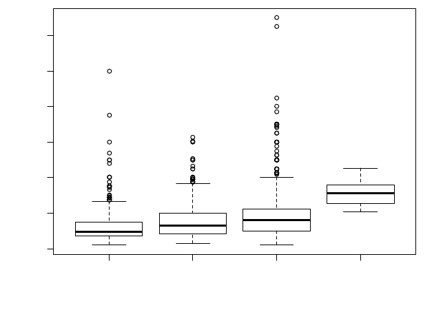
strategy by hosts. As figure 2 shows, average price increases with stricter cancellation
policies.
Figure 2.2: Boxplot of price by cancellation policy
To test if the impact of review varies by lodging segment, the SAR model was run
for each segment. Results in table 2.7 indicate that, except for moderate cancellation poli-
cy, the impact of quality on room price decreases as we move from flexible to super-strict
cancellation policy. The impact of quality on price for super-strict cancellation policy
flexible moderate strict super_strict_30
0 200 400 600 800 1000 1200
Cancellation Policy
Price

30
segment is not significant at 5% confidence level. Zhang, et al. (2011) found similar re-
sults when studying the determinants of hotel room prices. When considering lodging
segments, they found a positive impact of quality on room price for economy and mid-
scale hotels. However, for luxury hotels, quality does not affect room price. For the high-
er lodging segment, quality is no longer a differentiation factor. In Boston, all the hosts
who use a super-strict cancellation policy offer an entire home or apartment for rent on
the Airbnb platform. For these hosts, the quality of their room is already embedded in the
type of room they offer.
Table 2.7: Decomposition of the impact of review score for flexible, moderate, strict and
super strict cancellation policies
Segments
Impacts of review score
Direct
Indirect
Total
Flexible
0.015***
0.001***
0.016***
Moderate
0.003***
0.001***
0.005***
Strict
0.010***
0.001***
0.012***
Super strict
0.007*
0.000*
0.007*
Note: * denotes that the estimates are significant at 10% and ** and *** denote that they are significant at 5% and 1%
level.
Proximity to amenities has been shown to affect the price in hedonic price models
in previous studies. Our results indicate that only the distance to the nearest convention
center has the sign and significance level as expected. Participation in conferences for a
short-term period is among the reasons guests book rooms on Airbnb. The results of our
estimation support why hosts that are located closer to convention centers set higher pric-
es compared to hosts that are located further away from them. A one percent decrease in
the distance that separates a room from the nearest convention center leads to a 0.11 per-
31
cent increase in price. The distance to the closest train station does not affect price, as ev-
idenced by the non-significance of its coefficient.
Among the socioeconomic variables, the coefficients for education and income
per capita are positive and significant. We attribute the result to the theory of demand for
housing (Green and Hendershott, 1996). Neighborhoods with higher education and
income levels are more desirable, increasing the demand for houses in those
neighborhoods. High demand leads to high rental prices and consequently high prices for
the rooms rented on Airbnb. A one percent increase in the percentage of families with at
least a bachelor degree in the census tract where the room is located leads to a 0.09
percent increase in the room price. A similar change in income leads to a 0.07 percent
increase in price.
2.7. Sensitivity analysis
A series of alternative specifications are estimated for robustness checks. The es-
timation procedure is replicated with a linear mixed effects model. The same controls are
used as fixed effects variables. A random effect at the census tract level is added to char-
acterize idiosyncratic variation that is due to census tract differences. The census tract
might be a source of non-independence that needs to be considered within the model. We
test for the significance of the spatial lag price and review score variables using likeli-
hood ratio tests. P-values are obtained, and a likelihood ratio test is performed on the full
model with respect to the spatial lag price and with respect to the review score against the
model without these variables. The lme4 package (Bates, et al., 2015) is used in the es-
timation of the linear mixed model estimation. Table 2.8 presents the log-likelihood ratio
test results.

32
Table 2.8: Likelihood ratio tests for the statistical significance of price lag and quality
variables in the linear mixed effects models
Estimates
AIC
BIC
LogLik
Deviance
Chi-
square
Test for lag
price
Model without price lag
1069
1170
-516
1033
Model with price lag
0.25
1039
1146
-500
1001
31.82***
Test for quali-
ty
Model without quality
1083
1184
-523
1047
Model with quality
0.007
1039
1146
-500
1001
45.92***
Note: * denotes that the estimates are significant at 10% and ** and *** denote that they are significant at 5% and 1%
level.
The results of the linear mixed effects models confirm the spatial autoregressive
model results. The spatial lag price affects price (χ2 (1) = 31.82, p=0.000), increasing it
by about 0.33 ± (0.05). The review score also affects room price (χ2 (1) = 45.92,
p=0.000) increasing it by 0.01 ± (0.001). The coefficients for both review score and lag
prices are consistent with our assumption. Prices are strategic complements, and hosts
with rooms of high-quality set higher prices compared to hosts of low-quality rooms.
The full SAR specification regression is also estimated with 3 and 5 miles as
weight matrices. Increasing the threshold of the weight matrix allows the hosts to have a
larger number of competitors. The results of the estimates are presented in table 2.9. The
sign of the estimates for both the review score and the spatial lag price is consistent with
the results obtained using 1 mile as a weight matrix. The size of the spatial lag coefficient
estimates in the 3 and 5 miles weight model are lower than its size in the 1-mile weight
model, indicating, not surprisingly, that competition between hosts decreases as we in-
crease the distance between them. Hosts located further away from each other compete
less.
33
Finally, for a sensitivity check, other measures of quality are considered. First, we
use a unidimensional measure of quality that measures the overall satisfaction of the
guests. The unidimensional measure is similar to the single rating score commonly used
on many online platforms. Second, we consider six disaggregated measures of quality,
which are ratings by guests of specific aspects of the services provided by their hosts.
These measures are accuracy, cleanliness, check-in, communication, location and the
value of the apartment. The quality measure related to the accuracy of the listing reflects
how accurate the description of the apartment on the Airbnb platform is compared to the
guest’s experience. The quality rating cleanliness evaluates the cleanliness of the property
including the rooms, bathrooms and common areas. The quality of the check-in relates to
how welcome the guest felt when he/she first arrived.
Communications with the hosts as a quality measure provides an evaluation of
how long it takes the host to respond and the accuracy and usefulness of the host’s re-
sponses. A quality variable for the satisfaction of the guest about the location of the
apartment in the neighborhood and its proximity to amenities is also considered. The last
quality measure used for sensitivity check is related to the value of the listing, which
evaluates the guest satisfaction with paying the room rate for the service received.

34
Table 2.9: Estimates of the spatial lag regression with 3 and 5 miles as weight matrix
Variables
SAR
3 miles
5 miles
W_LnPrice
0.09**
(0.05)
0.14**
(0.05)
Intercept
3.86***
(0.56)
3.86***
(0.56)
Accommodate
0.12***
(0.01)
0.12***
(0.01)
Accommodate^2
-0.006***
(0.00)
-0.006***
(0.00)
Bathroom
0.08***
(0.01)
0.08***
(0.01)
Bedroom
0.17***
(0.01)
0.17***
(0.01)
Review score
0.01***
(0.00)
0.01***
(0.00)
Number of reviews
-0.002***
(0.00)
-0.002***
(0.00)
Room_type
Private Room
-0.43***
(0.01)
-0.43***
(0.01)
Shared Room
-0.68***
(0.05)
-0.68***
(0.05)
Cancellation Policy
Moderate
0.06***
(0.02)
0.05***
(0.02)
Strict
0.03
(0.01)
0.02
(0.01)
Super-strict
0.26***
(0.06)
0.25***
(0.06)
Log Distance
Convention
-0.14***
(0.00)
-0.15***
(0.00)
MBTA
-0.002
(0.01)
0.001
(0.01)
Education
0.09***
(0.01)
0.09***
(0.01)
Income
0.06***
(0.01)
0.06***
(0.01)
AIC
1121
1123
LM test for residual autocorrelation
7.26***
0.15
Note: * denotes that the estimates are significant at 10% and ** and *** denote that they are significant at 5% and 1%
level. Robust standard errors are in parenthesis
35
Results of the coefficients of these variables in the OLS and SAR regressions
(specified as in model IV with all the explanatory variables) are presented in table 2.10.
The results of the regressions of price on each of the different measures of quality show
consistent, positive and significant coefficients providing substantial evidence to support
the theoretical hypothesis that quality affects the price. The average impact of each of the
quality variables on the price was decomposed into its direct, indirect and total effect.
The results presented in table 2.11 show that for all the quality variables the average di-
rect effect on room price is higher than the indirect effect. Policies that provide an incen-
tive for hosts to improve the quality of their room have a direct positive impact on the
price of their room on Airbnb but also an indirect positive impact on the other hosts in
their neighborhood.
The size of the unidimensional measure of quality is significantly lower compared
to the other measures. Among the disaggregated measures of quality, cleanliness has the
highest impact on price (6.8 percent) followed by accuracy (4.9 percent). Value has the
lowest impact (3.2 percent). The impact of the unidimensional measure of quality on
price is less than one-third of the impact of value, the lowest disaggregated measure of
quality. This confirms Li and Hitt (2010) results where the unidimensional measure of
quality has been shown to be more associated with the product value than to its quality.
All the impacts (direct, indirect, and total) of the review score generated through senti-
ment analysis are closer to the impacts of the disaggregated measures of quality com-
pared to the unidimensional measure. This result suggests that sentiment analysis of the
reviews will better approximate quality than the unidimensional measure of quality and

36
using the unidimensional measure of quality will create a downward bias of the estimate
of the impact of quality on price.
Table 2.10: Impact of alternative measures of quality on price
Quality Variables
OLS
SAR
Review score
0.01***
(0.00)
0.01***
(0.000)
Unidimensional measure of quality
0.007***
(0.00)
0.006***
(0.00)
Accuracy
0.04***
(0.00)
0.04***
(0.00)
Cleanliness
0.06***
(0.00)
0.06***
(0.00)
Check-in
0.04***
(0.00)
0.04***
(0.00)
Communication
0.04***
(0.00)
0.04***
(0.00)
Location
0.03***
(0.00)
0.03***
(0.00)
Value
0.03***
(0.00)
0.03***
(0.00)
Note: * denotes that the estimates are significant at 10% and ** and *** denote that they are significant at 5% and 1%
level. Robust standard errors are in parenthesis
Table 2.11: Decomposition estimates of the direct and indirect effects of quality variables
on rooms' prices
Quality Variables
Direct
Indirect
Total
Review score
0.010***
0.004***
0.015***
Unidimensional measure of quality
0.006***
0.003***
0.010***
Accuracy
0.049***
-0.000***
0.049***
Cleanliness
0.068***
-0.000***
0.068***
Check-in
0.043***
-0.000***
0.043***
Communication
0.043***
-0.000***
0.043***
Location
0.036***
-0.000***
0.036***
Value
0.032***
-0.000***
0.032***
Note: * denotes that the estimates are significant at 10% and ** and *** denote that they are significant at 5% and 1%
level.
37
Among the quality variables, cleanliness has the strongest effect on the price of
the rooms, followed by accuracy. Cleanliness seems to be the most important quality
variable that affects price. This result is consistent with de Oliveira Santos (2016) who
studies more than 8000 hostels worldwide and identifies cleanliness, location, and facili-
ties as the main characteristics that explain accommodation prices. With the growth of
online platforms, where reviews can inform prospective guests, these qualities can affect
demand for hosts’ rooms.
38
2.8. Conclusion
Online reviews and ratings are largely recognized to impact consumers’ purchase
decisions especially on online platforms where they serve as proxy for quality of products
and services. Many studies in the hotel industry literature use rating or single review
scores to examine the relationship between quality and price. However, evidence from
the existing literature suggests that single rating measure can lead to biased conclusions
on the relationship between reviews rating and price since the single measure might not
represent the complexity of the customer opinion or sentiment about a good or service
accurately.
This article contributes to the literature on the impact of quality on price in the
hospitality industry. Contrary to the existing literature, where unilateral rating review as
scored by the guest is used as proxy for quality, this study relies on a novel approach to
derive the score in the reviews. With sentiment analysis, the opinions in the reviews are
extracted and scored to derive the total score of the review. This study also uses a spatial
hedonic price model to account for the spatial correlation of price data. Using data from
Airbnb platform, the results of the empirical analysis suggests that scores derived from
the sentiment analysis of the reviews are better indicators of quality than single rating
scores.
Although disaggregated multidimensional components of quality such as cleanli-
ness, accuracy, communication, location, are better predictors of the listing price than the
reviews, the latter is still a better proxy for quality than unidimensional rating scores. Re-
views reveal information about the intrinsic quality of the hosts and these reviews affect
the demand on the Airbnb platform. The reviews affect not only the host price but also
39
the price of other neighboring hosts. The policy implication for Airbnb is to create incen-
tives or policies for hosts to improve the quality of their listings. This will have spillover
effects on the price set by other hosts. Cleanliness of the property and accuracy of the
listing are the two most important quality measures that affect price and the policies
should be directed towards improving those qualities.
The theoretical model suggests that when a host increases its price, its rivals also
increase their price, making them strategic price complements. The results of the
empirical analysis support the theoretical framework. Other factors, such as the number
of bedrooms and bathrooms, as well as the number of people a room can accommodate,
also have a positive effect on the price set by the owners.
40
CHAPTER 3 CHAPTER 3. TEXT-BASED PREDICTIONS OF BEER
PREFERENCES BY MINING ONLINE REVIEWS
3.1. Abstract:
There is an increasing interest in categorizing texts using the words used to write
the text. The process involves decomposing the texts into the words composing them and
using the frequency of those words to predict the text polarity. The text categorization
approach may use single words composing the texts or longer combinations of the words.
Longer combinations of the words have the advantage of better representing the complex-
ity of human language compared to single words. Moreover, less frequent terms may also
better discriminate between reviews than more common words.
This study tests these two hypotheses in the context of beer reviews. It shows that
the words used in the reviews can be used to predict consumer’s preferences for beer.
Moreover, it shows that the use of less frequent terms in the predictive models outper-
forms the use of more frequent terms. This confirms Sparck Jones (1972)’s heuristics re-
sults. However, low-level combinations of the words in the reviews better predict con-
sumers’ preferences compared to high-level combinations even though the latter better
represent the complexity of human languages.
3.2. Introduction
With the advent of the web 2.0, user-generated-content (UGC) such as reviews
and comments for online products and services are being generated at an increasing rate
and are accessible to a large audience on the internet. On online platforms, consumers are
encouraged to share their experience about various aspects of the products or services
41
(Yu, et al., 2011). The multiple reviews, comments, and rating left by the consumers car-
ry important about their opinions of the products. Prospective consumers consider this
information as a form of collective evaluation of products and services quality by previ-
ous consumers (Chen, et al., 2008). They search the reviews for specific features of the
products and form their opinion based on the evaluation of the features by previous con-
sumers. The presence or absence of specific features in reviews can affect consumers’
purchasing decision, suggesting an underlying relationship between the features and the
perceived quality of online products or services.
In the last few years, UGCs have received a lot of interest in economics. Senecal
and Nantel (2004) show that online product recommendations influence consumers’
choice. Chen, et al. (2008) show that reviews that are found more helpful have a stronger
effect on consumers’ choice. Zhang, et al. (2013), Luca (2016), and Floyd, et al. (2014)
examine the positive influence of online reviews on product sales. These studies rely on
methods that can extract value from the UGCs and their relationship with product charac-
teristics. For example Schumaker and Chen (2009) use a combination of linguistic, finan-
cial and statistical techniques to predict stock prices. Archak, et al. (2011) uses textual
representation or text categorization to identify the product features that influence prices.
In recent years, using text categorization, many studies have investigated the association
between the features in the reviews and the other measures of quality such as numeric
rating, thumbs up or thumbs down, and star rating.
Text categorization relies on unigram or n-gram representations of the reviews to
predict the review score. A unigram is the result of the decomposition of text into the sin-
gle words used to write the text. Bigrams, trigrams, and n-grams correspond to a decom-
42
position of the text into two, three and n-words, respectively. Bigrams correspond to a
higher-level representation of the text compared to unigram and a lower-level representa-
tion compared to trigram. Low-level n-gram representations do not account for the com-
plexity of the human language. For example, unigrams cannot capture the relationship
between two words such as a word and its negation (i.e., “good” vs. “not good”) or a
word and its modifier (i.e., “flavored” vs. “barely flavored”). Bigrams can capture these
relationships but not the meaning of larger expressions. Conversely, larger n-grams can
effectively represent longer expressions but do not occur as often in many reviews. A
word such as “flavor” or an expression such as “best flavor” are more likely in reviews
than an expression such as “certainly the best-flavored beer. “
For an n-gram representation of an expression such as “certainly the best-flavored
beer” different combinations of the words in the expression will be examined. Few ex-
amples of these combinations for a quad-gram are: “certainly best-flavored beer”, the
original sentence, but also “best-flavored beer certainly”, “certainly beer best-flavored”,
etc. Only the original sentence is likely to be present in only one review. Its frequency for
that review is one and zero for the other reviews. The use of larger expressions in an n-
gram representation of the reviews introduces sparsity in the data generated from decom-
posing all the reviews into n-grams. In such sparse data, some reviews have zero occur-
rences for the n-gram representation. Text categorization tasks with sparse data require
computationally intensive methods capable of identifying and extracting relevant features
capable of predicting reviews’ scores or polarity (positive or negative reviews). This pa-
per addresses the problem of predicting consumers’ preferences for beer using n-grams
representation of the reviews left by the consumers online. The n-grams represent the
43
beer features associated with consumers’ preferences expressed as rating scores (consum-
ers rate the products on a scale ranging from 0 to 5). Using a machine learning algorithm,
the random forest, we examine the performance of unigrams, bigrams, and trigrams in
predicting consumers’ preferences. We compare two approaches. One uses the frequency
of the most frequent n-grams (unigrams, bigrams, and trigrams) to predict consumers’
preferences. The second uses the least frequent n-grams representations of the reviews
(inverse frequency). The results show that inverse frequency method better discriminates
between the reviews in predicting consumers’ preferences.
The remainder of the paper is organized as follows. Section 2 presents the litera-
ture review of text categorization. Section 3 provides the methodology used to extract the
features, select the relevant ones and perform the preferences’ prediction using random
forest. The results are presented in section 4, and section 5 concludes.
3.3. Literature review
Text categorization consists of using text contents to identify predefined catego-
ries. This method has received a lot of interest in many fields such as machine learning
and computational linguistics (Lewis, et al., 2004). In machine learning, text categoriza-
tion involves building a learner capable of identifying the class of a specific text among
many predefined categories (Zhang and Zhou, 2006). A couple of decades ago, text cate-
gorization tasks were performed manually. Han, et al. (2001) reports that in 1999 a com-
pany such as Yahoo used human experts to categorize online documents. Manual catego-
rization of online texts is time-consuming and prone to errors. The growth of the internet
has limited the volume of materials that can be manually categorized. Online contents are
growing in size and diversity. Businesses collect trillions of bytes of data on their ser-
44
vices (Domingos and Hulten, 2000, Sati, 2017). IBM (2017) reports that 2.5 quintillion
bytes of data are created every day. The growth of the internet has also eased the release
online of published information by millions of content creators (Larson, 2010). Handling
these volumes of online contents manually as Yahoo did in 1999 (Han, et al., 2001)
would be challenging.
Several computational based methods have been explored to perform the text cat-
egorization task. The methods, which vary from machine learning to numerical methods,
consider the text as semi-structured data. Some methods use variations that are statistical-
ly detectable in style to classify documents based on their source style (Biber, 1991).
Other methods exploit the features in the texts to identify their genres (Finn, et al., 2002).
A conventional approach consists of using the bag of words (BOW) representation of
texts. In the BOW, the words in the texts represent features so that each text is evaluated
depending on the presence or absence of the word. The frequency of the occurrence of a
word in the texts is used to assign them to predefined classes. The words are the attributes
of the text and the basis for the categorization task. The vector resulting from the decom-
position of a text into the single words used to write the text is called unigram. Bigrams,
trigrams and n-grams correspond to the vectors equivalent to the decomposition of the
text into two, three and n-words, respectively. For example, a review that contains an ex-
pression such as “best-flavored beer” would be decomposed into the following unigrams:
“best”, “flavored”, and “beer”. For each of the unigrams, the reviews will be scored 1 if
the unigram is present and 0 otherwise. Reviews that have two occurrences of the uni-
gram “beer” have a frequency equals to 2 for this unigram. A bigram representation will
examine the presence or absence of the two-words combinations of the words used in the
45
expression in each review. The two-word combinations are "best flavored”, “flavored
best”, “best beer”, “beer best”, “flavored beer”, and “beer flavored”. Each review is eval-
uated based on the frequency of the bigrams.
The BOW approach applied to reviews poses two main problems. First, the words
do not appear equally in all the reviews since the online content creators write the re-
views independently from one another. This generates large sparse matrices where some
words appear only once or a few times in the reviews. Categorization of text in large
sparse matrices is a computationally intensive task. The second problem related to low-
level BOW approach is the complexity of human language that is not captured by the
low-level n-gram representations. A single word outside of its context can be ambiguous
regarding its polarity. Yet, combinations of words tend to be less ambiguous and better
capture the polarity of the sentences (Bespalov, et al., 2011). For example, it is difficult to
identify the polarity of a unigram such as “impressive” compared to a bigram such as
“not impressive” that is composed of the previous unigram and a modifier. High-level n-
gram representations have been shown to perform better than low-level representations in
text categorization (Cui, et al., 2006). Cui, et al. (2006) indicate that text classifier algo-
rithms that use high-level n-grams representation (n=3,4,5,6) outperform algorithms that
use unigrams and bigrams. However, high-level n-gram representations exacerbate the
matrix sparsity problem since longer combinations of words are less frequent in the re-
views than each of the words of the combinations.
The sparsity of the BOW approach can be addressed by reducing the number of n-
grams used to perform the text categorization task. Yet the features selection method can
result in the suppression of features relevant for the classification task. Sparck Jones
46
(1972) shows that terms that occur in many documents are less effective in discriminating
between the documents than less frequent terms. He proposes a method that allocates
more weight to less frequent terms: the inverse document frequency weighting. Inverse
document frequency, which has its origins in heuristics (Balinsky, et al., 2010), is com-
monly used in information retrieval Metzler (2008). This weighting method handles
sparse matrices by stressing discriminative features and reducing the influence of irrele-
vant ones (Meyer, et al., 2008). Discriminative terms or features are the ones that do not
appear in many documents and whose inverse document frequencies are high (De Vries
and Roelleke, 2005). Greiff (1998) uses the relationship between document frequency
and the mutual information between relevance and term occurrence to sketch a theoretical
explanation of the improved retrieval performance of inverse document frequency for
term weighting. The inverse frequency weighting method can also be effective in finding
relevant small sets of terms that can be effective in building predictive models.
Text categorization applications have also been used in economics research.
Haag, et al. (2000), Goodwin, et al. (2014), and Nowak and Smith (2017) use textual in-
formation to address the omitted variables bias problem that plagues many hedonic pric-
ing models. Schumaker and Chen (2009), Schumaker and Chen (2009), and Hagenau, et
al. (2013) show the importance of textual representation of news in predicting stock pric-
es. Text categorization techniques can also be effective in marketing for brand position-
ing, or product development. Yu, et al. (2011) for example, use this method to identify
the most important product features to consumers. They use this approach to develop an
aspect-ranking algorithm that extracts the important aspects of 11 popular products. Ap-
47
plied to document categorization this approach improves the classification performance
considerably.
Due to the importance of text categorization in classifying reviews, this study ex-
amines its use in the food industry to identify consumers’ preferences or perform task
such as sensory analysis. In the food and beverage industry, sensory analysis is often used
to evaluate a product based on its perceived sensory characteristics (Murray, et al., 2001).
It requires the selection, training, and maintenance of a panel of judges that assess prod-
ucts by evaluating their qualitative and quantitative sensory components (Murray, et al.,
2001, Stefanowicz, 2013). The panel decides the features of products that best represents
their similarities and dissimilarities, agree on the assessment method of the features, pro-
ceed to training on a sample of products before assessing the group of products of interest
through a randomized experiment (Varela and Ares, 2012). In the last decade, various
methodologies and techniques have been developed to overcome the time and complexity
of classic sensory analysis techniques (Varela and Ares, 2012). This study proposes a
novel approach: text categorization. It evaluates how product features in online reviews
and comments can be used to predict consumers’ preferences for beer.
3.4. Methodology
We decompose the problem of predicting consumers’ preferences for beers with
the content of the reviews as a three-step procedure. First, we use the bag-of-words
(BOW) approach to extract the terms or features in each review. Second, we remove fea-
tures that would be irrelevant for the predictive model. Third, we use a random forest as a
supervised machine-learning algorithm to predict consumers’ preferences with the ex-
tracted features.
48
3.4.1. Feature extraction
Reviews were collected between September and October 2017 from BeerAdvo-
cate (BA), an online community of beer enthusiasts and professionals. The members of
the community share their opinion and experience about beers through reviews and
comments on this online platform. Reviewers also rate each of the beers based on their
satisfaction. The rating score ranges from one to five. The Python programming language
was used to scrape the reviews and the scores from the website. A total of 5500 unique
reviews were scrapped from BeerAdvocate. A BOW feature extraction approach is ap-
plied to the reviews.
The BOW approach, commonly used in natural language processing models,
identifies and extracts features in a set of documents or corpus. Here, the collection of
reviews constitutes the corpus. Punctuations, unnecessary words and characters are re-
moved from the corpus. The corpus is then decomposed into its unique words to form a
vocabulary. The occurrence of each word in the vocabulary for each review is scored to
form a term-document matrix. In the term-document matrix, the rows correspond to the
reviews in the corpus and the columns to the words or terms in the vocabulary. The cell
values are the frequency attached to the word or term in the review. For example, the cell
(i, j) is the frequency of occurrence of the term i in the review j.
Two datasets are derived from the term-document matrix: one dataset with the
most frequent terms (the term-document matrix) and another with the less frequent terms
(the inverse term-document matrix). More frequents terms in multiple reviews might not
convey enough information to discriminate between the reviews contrary to less frequent
(Popescu and Etzioni, 2007). Less frequent words can be specific to certain categories.
49
Their presence in reviews can better contribute indicate similarities between those re-
views compared to words that are more frequent. For example, a word such as “malt” is
more likely to be present in most beer reviews since most beers are made out of malt.
Contrary, a word such as “citrus” is less common to all beer. Few beers have a citrus
taste. Thus, in addition to the frequency of the term in the cell, we also use the inverse of
the frequency for comparison. The inverse weighting technique assigns more weight to
less frequent terms.
We also use higher-level n-grams in the vocabulary. This method has the ad-
vantage of capturing meaningful terms or expressions in the predictive models. For ex-
ample, even though malt is used in most beer, the origins of the grains used as malt can
affect the percentage of alcohol, the flavor, and aroma. Barley is the most common grain
used for malting. Malt can also be derived from wheat and rye. Instead of using a uni-
gram such as “malt’, bigrams such as “malt barely”, “malt wheat” and “malt rye” are bet-
ter at categorizing the different types of beers. Three different types of datasets are de-
rived based on the vocabulary used: unigrams, bigrams, and trigrams. Unigrams corre-
spond to a dictionary with single words or terms. Bigrams and trigrams correspond to re-
spectively two and three terms. Through the combination of the three types of n-grams
dictionaries and the two types of term-document matrices six datasets were generated.
3.4.2. Feature selection
The feature extraction procedure described above produces sparse datasets since
some terms appear in only a few reviews. These terms or features, referred to as zero var-
iance predictors or near-zero variance predictors, do not perform well in predictive mod-
els and might create errors in the computation (Kuhn and Johnson, 2013). Some of the
50
features might not be relevant in explaining the consumers’ preferences or might be re-
dundant. Moreover, when the number of variables introduced in a machine-learning
model is too large, many machine learning algorithms loose accuracy. This issue is com-
monly known as the minimal-optimal problem (Nilsson, et al., 2007). A feature selection
solution helps deal with the minimal-optimal problem by selecting the minimum number
of relevant features needed to yield the best predictive models.
To address the minimal-optimal problem, many algorithms have been developed.
According to Fonti and Belitser (2017) these algorithms can be classified into three gen-
eral categories: filter methods, wrapper methods, and embedded methods. Filter methods
use a statistical measure to rank the features and select high scoring features for model-
ing. Some examples of filter methods are ANOVA tests, Chi-squared tests, and correla-
tions. Wrapper methods work on the feature selection as a search task. They build differ-
ent subsets of the features and use the subsets to perform a predictive task. The subset
that yields the best performance for the predictive task contains the selected features. The
search task may be heuristic (forward, backward, or recursive with features elimination),
or based on a particular methodology (best-first search), or even randomly determined
(hill-climbing algorithm). Finally, embedded methods are a combination of the two pre-
vious methods.
To select the minimal features that will give the best prediction results among the
set of n-grams explanatory variables, the Boruta algorithm (Kursa and Rudnicki, 2010) is
implemented. This algorithm is a wrapper method that is based on recursively finding all
relevant variables while getting rid of the features that don’t perform well. Table 3.1
summarizes the number of features selected with the Boruta algorithm.

51
Table 3.1: Number of features selected with the Boruta algorithm
Number
of reviews
Number of attributes con-
firmed important
Number of attributes
confirmed unim-
portant
N-
grams
Unigram
5500
107
663
Bigram
5500
27
253
Trigram
5500
6
26
N-
grams
inverse
Unigram
5500
116
654
Bigram
5500
24
256
Trigram
5500
6
21
3.4.3. Predictive model: the random forest
The objective is to classify consumers’ preferences based on the features repre-
sented by the words used in their reviews. To solve this supervised
4
classification prob-
lem, an ensemble learning algorithm, the random forest introduced by Breiman (2001) is
used on the six n-grams datasets. The random forest model was compared to other ma-
chine learning models such as the linear discriminant analysis, the support vector ma-
chines, and the K nearest neighbors (KNN). The random forest performs better than the
other models in predicting consumers’ preferences. Ensemble learning algorithms such as
random forest are a collection of single classifiers, tree-based classifiers in the case of the
random forest, combined into one model. Ensembles often perform better than individual
4
Machine learning that uses input data (independent variables) to predict an output (dependent varia-
bles) are supervised machine learning models. Those that use and input with no corresponding output are
unsupervised machine learning models.
52
classifiers. Breiman (1996) shows that ensembles have a lower variance relative to the
single classifiers that compose them. Each of the single classifiers is selected inde-
pendently of the others, which makes ensembles more accurate and robust to noise than
single classifiers (Breiman, 1996, Breiman, 2001, Dietterich, 2000). This accuracy and
robustness to noise explain the interest they have received in the literature. The main
steps to build the RF classifier are summarized as follows:
Step1
The rating scores are binned into two categorical variables. Reviews scores of 4
and below (included) are categorized as “Good” reviews; those greater than 4 are catego-
rized as “Very Good” reviews. We do not attribute the good and very good attributes to
the two categories, and these attributes are not understood as such. The choice of the two
categories is for simplicity and to ensure that the dataset is balanced. The “good” and
“Very Good” categories represent, respectively, 51.59% and 48.41% of the dataset. The
5500 observations in the dataset are split into two sets: a training sets and a test set. For
each of the n-gram dataset, the training set, composed of 80% of the observations, is used
to train the classifier. The remaining 20% of the observations comprises the test set,
which is used to evaluate the performance of the classifier. Since the test set is unknown
to the random forest classifier, we can assess the capacity of the classifier to predict the
class of the observations in the test set correctly. Each random forest classifier is trained
with a training set but tested on the test set.
The random forest creates n
using recursive partitioning of the initial training
data, D =
{
X
; Y
}
…
, and combines their results. Each tree contains a sample D
(ran-

53
domly selected with replacement) of the initial data D. In other words, the tree j is a sub-
set of the initial training set which contains a randomly selected D
= X
; Y
sample of
D. Because the random selection is with replacement, without deletion of the data select-
ed from the training data set, some data may be part of many trees while other might nev-
er be used in any tree.
Step 2
Each tree j with a sample D
of the training set performs its classification inde-
pendently. Each decision tree is in itself a classification task. At each node in a tree, f
F features are randomly selected among the F features available. At that node, the best
binary split is used to partition the node. Each “parent” node is split into two homogenous
“child” nodes. Gini impurity I (Menze, et al., 2009) measures node homogeneity. It is
given by:
I = 1
(
)
with n
the number of objects in class c at node n.
The lowest Gini impurity value computed among the f features will guide the choice of
the splitting criterion at the node. Each decision-tree classification task j is associated
with a classification error Err
that measures the misclassification rate.
Err
=
1
|D
|
I(y
y
)
D
is the remaining dataset in D not selected in the bootstrap samples D
. The subset D
is
called out-of-bag (OOB) and is defined as D = D
D
. |D
| is the size of the j
OOB
54
subset, y
is the predicted class using the tree j classification on an observation i not in the
random bootstrap sample selected D
.
The same process is repeated for each of the bootstrap samples (trees) in the training data
D. The trees are combined to form the random forest classification model. To predict the
class of an observation, the model uses the vote of each decision tree for each class. The
final predicted class will be the class that will obtain the majority of the votes.
10-fold cross validation is also used to reduce the model overfitting using the model ac-
curacy as a control metric. The training set is divided into ten reduced sets. The model is
trained using nine of the reduced sets as training data, and the subsequent model is evalu-
ated on the remaining part.
Step 3
Once step 2 is used to grow each decision tree, then the random forest model is
tested with the test set to assess the performance of the random forest classifier. By using
the test set, which was not used to train the random forest classifier, we can evaluate the
capacity of the classifier to correctly predict the class of observations in the test “never
seen” by the classifier. To predict the class, “Good” or “Very Good,” of an observation
(review), the model relies on the vote of each decision tree. The class that obtains the ma-
jority of votes is retained by the random forest classifier as the predicted class. However,
the classifier may wrongly classify the classes. Models that accurately predict the classes
of the reviews are preferred to those with large misclassifications errors.
Three performance criteria serve for the evaluation of the models. These criteria
depend on the number of correctly classified observations, true positives (reviews that are

55
“Good” and correctly predicted by the model as such), denoted by TP, and true negatives
(reviews that are “Very Good” and correctly predicted as such), denoted by TN. There
are also false positives (reviews that are “Very Good” but falsely predicted as “Good”),
denoted by FP and false negatives (reviews that are “Good” but falsely predicted to be
“Very Good”), denoted by FN.
The first performance criterion is the accuracy, the percentage of correctly pre-
dicted “Good” and “Very Good” preferences. The accuracy criterion reflects the capacity
of the model to predict the “true” class of the reviews correctly based on the n-grams. It is
given by the formula:
Accuracy =
TP + TN
TP + TN + FP + FN
The second performance criterion is Cohen (1960)’s Kappa statistic which helps
evaluate each model, but also compares the models amongst themselves. The Kappa sta-
tistics compares observed accuracy with the expected accuracy that might occur by
chance if the classes were randomly guessed. The Kappa statistic is given by:
Kappa =
Observed Accuracy Expected Accuracy
1 Expected Accurary
Kappa values vary between zero (0) and one (1). Kappa values greater than zero indicate
a classifier that achieves a rate of classification that exceeds chance levels.
The third performance criterion that is used is the Area Under the Curve (AUC).
It is a function of the sensitivity or true positive rate (TPR) and specificity or false posi-
tive rate (FPR) of the model.

56
True Positive Rate =
TP
TP + FN
False Positive Rate =
TN
TN + FP
The sensitivity or true positive rate measures the proportion of “Good” reviews
that are correctly predicted to be “Good” among all “Good” reviews. Conversely, the
false positive rate measures the proportion of “Very Good” reviews that are wrongly pre-
dicted to be “Good” among all “Very Good” observations. A model with a high TPR is
less likely to misclassify “Good” observations. However, a model with a high FPR is
very likely to misclassify “Very Good Observations”.
What is the probability that the random forest model ranks a random sample of
“Good” observations better than a randomly chosen sample of “Very Good” observa-
tions? A graph of the TPR against the FPR at different probability thresholds gives the
Receiver Operating Characteristic (ROC) curve. A ROC graph that fits exactly on the di-
agonal corresponds to a random predictor and the model that generates such graph is as
good as a coin toss. In contrast, a model that would yield at different probability thresh-
old settings TPR=1 and FPR=0 will have a ROC at the left corner of the graph (coordi-
nate (0,1)). A model with such ROC has 100% TPR and 0% FPR. Such a model corre-
sponds to a perfect classification model. In practice, such models are rare but the closer
the models are to the left corner, the better they predict, and the distance that separates
the model from the diagonal represents how well the model is at the classification task
compared to a random guess. The area under the ROC curve (AUC) is used as the second
criteria to evaluate the model's performance. The AUC gives the probability that a ran-
57
domly chosen “Good” observation is classified as a “Good” observation, rather than a
randomly chosen “Very Good” observation. The diagonal corresponds to an AUC of 0.5
and the perfect classification model corresponds to an AUC of 1. Most models will have
an AUC between 0.5 and 1.
3.5. Results and discussions
3.5.1. N-grams representation
To predict consumers’ preferences for beer using an n-grams representation of the
review, we apply the proposed methodology of a random forest classification algorithm
to the six datasets. The six models represent the use of six different n-grams dependent
variables. The rf-unigram model is the algorithm related to the dataset represented by the
most frequent unigrams. The rf-unigram-inv is the algorithm related to the dataset that
contains the less frequents unigrams. Similarly, rf-bigram, rf-trigram, and rf-bigram-inv,
and rf-trigram-inv are the algorithms related to more frequent bigrams, trigrams and less
frequent bigrams and trigrams, respectively. Figure 3.1 compares the models based on
their accuracy to predict consumers’ preferences and the Kappa statistic. Table 3.2 pro-
vides the details of the accuracies and Kappa values.
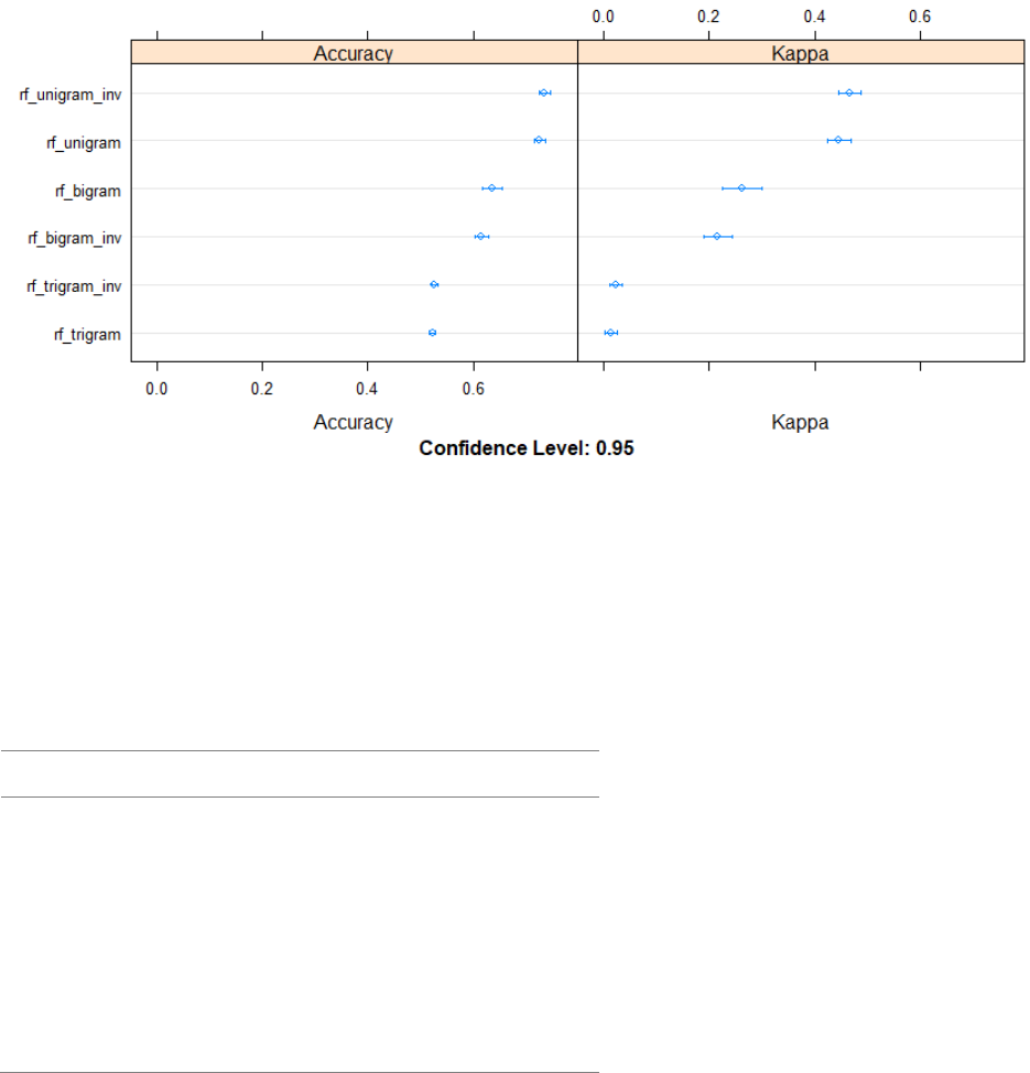
58
Figure 3.1: Performance comparison of the unigram, bigram, trigram models and their
inverse
Table 3.2: Models accuracy and Kappa statistic
Models
Accuracy
Kappa
Uni-gram
0.72
0.44
Bi-gram
0.63
0.26
Tri-gram
0.51
0.01
Uni-gram-inverse
0.73
0.46
Bi-gram-inverse
0.59
0.21
Tri-gram-inverse
0.52
0.02
Examination of the model's accuracies indicates that almost all the random forest
models perform better than the random choice baseline of 50%. Only the trigram and the
trigram-inverse models, with an accuracy of 51% and 52%, respectively, have a predic-
tive power almost identical to the random choice baseline of 50%. With accuracies of
59
72% and 73%, the unigram and unigram-inverse models perform well in comparison to
the other n-gram models. The bigram and bigram-inverse models follow. The model ac-
curacy is reduced by 9 percentage points when we move from a unigram to a bigram
model and by 21 percentage points when we use a trigram instead of a unigram. Contra-
ry to our expectation, the unigram model, which is a low-level n-gram representation of
the reviews, has a better predictive power than higher representations such as the bigram
and trigram models. Even though high-level n-gram representations account for the com-
plexity of the human language, their use to predict consumers’ preferences is less accu-
rate than low-level n-gram representations in the case of beer reviews. Contrary to the
rest of the literature, our result is consistent with Pang, et al. (2002)’s sentiment classifi-
cation study using machine learning. They also report a decline in accuracy when switch-
ing from unigram to bigram models suggesting that bigram models are not that effective
in accounting for the reviews’ context. However, a common characteristic of Pang, et al.
(2002)’s study and ours is the small size of our dataset. Pang, et al. (2002) use 2053 re-
views for their classification and we use 5500 reviews. Chu, et al. (2012) shows that larg-
er sample sizes improve classification accuracies. Our result might have been different
with a larger sample size. Cui, et al. (2006) segments use 100,000 product reviews in
classifying text. Their result confirms the higher performance of models that use high-
level n-grams representations.
3.5.2. Term frequency vs inverse document frequency
The second objective of this study is to evaluate the performance of the predictive
models when using less frequent terms to discriminate between the reviews. From figure
1 and table 2, except for the bigram models, the use of the inverse document frequencies
60
in the unigram and trigram models improve the model's accuracies by 1 percentage point.
Although the accuracy gain is not substantial, this result confirms that in two out of the
three of the n-gram models considered in this study, the prediction of similar consumers’
preferences for beer can be improved with the use of inverse document term frequency.
Analysis of the Kappa statistics is consistent with the analysis of the accuracy
values. The remaining results and discussion are centered around the performance of the
best predictive model, the random forest with the unigram inverse document frequency.
3.5.3. Performance analysis of the random forest classifier for the unigram-inv model
The final random forest model built with the unigram inverse document frequency
uses 500 trees and achieves an OOB error rate estimated at 27.33%. To examine the pre-
dictive performance of this model, we tested the model on the 1099 observations (re-
views) in the test set. By construction, the test set is “unseen” by the random forest classi-
fication model since it is independent from the training set used to build the model. Table
3.3 displays the confusion matrix.
Table 3.3: Confusion matrix of the unigram-inverse random forest model
Reference
Prediction
Good
Very Good
Good
478
195
Very Good
89
337
61
The unigram-inverse random forest model reaches a sensitivity or positive rate of
84.30% and specificity or false positive rate of 63.45%. These results indicate that the
unigram inverse random forest model is better at identifying the reviews classified as
“Good.” However, the approach used when binning the data could lead to this difference
in class prediction. Data categorized as “Good” cover a larger interval ([0, 4]) compared
to data categorized as “Very Good” (]4, 5]).
The Operating Receiving Characteristics (ROC) curve (figure 3.2) derived from
the sensitivity and the specificity values confirms that the unigram inverse random forest
model built performs better than a random strategy in separating “Good” preferences
from “Very Good” ones. The ROC curve showing the trade-off between sensitivity and
specificity also identifies the best threshold for separating the “Good” and “Very Good”
preferences. This threshold is the value that maximizes the Youden’s index independently
from the percentage of the two preferences classes.
Youden’s index = sensitivity + specificity -1.
For the unigram inverse random forest model, the threshold is given by the point
that corresponds to a specificity of 73.9% and a sensitivity of 77.4%.
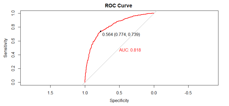
62
Figure 3.2: Receiver Operator Curve (ROC) and Area Under the Curve (AUC) for the
unigram-inverse random forest model
3.5.4. Effect of number of trees on the model accuracy
In step 2 of the random forest classifier, each decision tree constitutes a classifica-
tion task. The out-of-bag (OOB) sample is used as a test set to evaluate the error generat-
ed by each decision tree classification task. The OOB error rate estimate is the percentage
of wrong classifications. Recall that the OOB observations are not used to build the tree.
They constitute valid test sets for the trees. The error of each tree in predicting the OOB
observations averaged over all trees give an estimate of the OOB error rate. By construc-
tion, this OOB error rate is an unbiased estimate of the random forest model. Figure 3.3
presents the effect of the number of trees on the OOB error rate estimate. The figure
shows that as the number of trees grows the OOB error rate decreases, flattens out and
converges around 200 trees. Additional trees beyond 200 trees do not improve the mod-
el’s error rate. The two other graphs show the error in classifying the “Good” and “Very
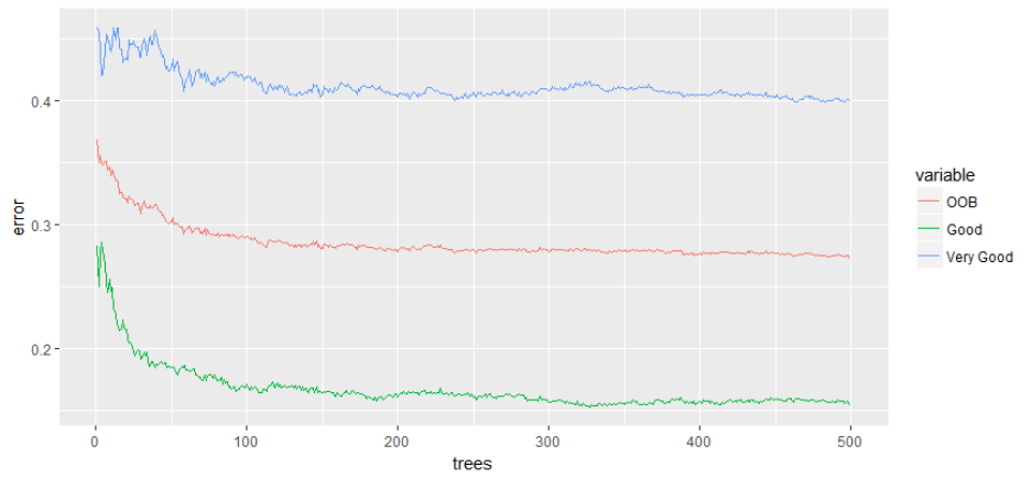
63
Good” classes. The effect of the number of trees on the error rate with these two classes
follows the same pattern as the effect of the number of trees on the OOB error rate. This
result suggests that we can reduce the computational time of our model by using approx-
imately 200 trees.
Figure 3.3: Effect of the number of trees on Out of Bag, Good, and "Very Good" catego-
ries error rate estimates
3.5.5. Identification of the most important features in the reviews
To decide whether or not a feature will be used in a tree to partition a node, the
random forest algorithm uses the Gini Impurity Index I (Breiman, 2017). When a split is
made at a node, the parent node has a higher Gini index compared to its two descendants.
The importance of a feature is evaluated by adding the decreases in the Gini index at all
the nodes in the forest where the nodes are partitioned using that feature. Figure 4 pre-
64
sents the most important features based on their mean decrease for Gini. Examination of
figure 3.4 shows that the features that better discriminate consumers’ preferences are re-
lated to the smell or taste (vanilla, oak, citrus, grapefruit), look (clear, juicy), and overall
quality of the beer (great, good, perfect).

65
Figure 3.4: Importance of the features in the unigram inverse predictive random forest model
3.6. Conclusion
This study presents a machine learning method to predict consumers’ preferences
for beer using text categorization of consumer reviews. Text categorization is commonly
used in many fields such as computational linguistics, economics, and finance. For prod-
uct development and brand positioning, marketers are interested in product features that
can better express consumers’ preferences for their products. They usually refer to senso-
ry analyses that can be costly and time-consuming. This study examines how product fea-
tures in online reviews and comments can be used to predict consumers’ preferences.
The study compares two approaches. First, it evaluates the performance of low-
level n-grams representation of reviews compared to high-level n-gram representations.
Contrary to low-level n-gram representations, higher-level representations can capture the
relationship between different words accounting for the complexity of the human lan-
guage. Second, the study tests whether the use of less frequent terms in reviews better
discriminates between the reviews than more common terms. Using the random forest
algorithm, our analysis shows that in the case of beer reviews posted by beer enthusiasts
on an online platform, low-level n-gram representation of the reviews outperforms higher
levels n-gram representations. Model accuracy is reduced as higher-level ones replace
low-level representations. However, our analysis confirms Sparck Jones (1972)’s heuris-
tics results that terms which occur in multiple documents are less effective in discriminat-
ing between the documents than less frequent terms. By allocating more weight to the
less frequent terms in our models, we are able to increase their predictive performance.
Finally, our analysis identifies beer attributes related to the smell or taste, look, and over-
67
all quality of the beer as the most important features in predicting consumers’ prefer-
ences.
This study shows that there is a value in online reviews and there are ways to use
those reviews beyond simple numerical ratings. Important product features in evaluating
consumers’ preferences for the product can be extracted from online reviews written
about the product. Improving models for predicting consumers’ preferences with the re-
views online, can significantly contribute to product development and brand positioning
by marketers.
68
CHAPTER 4 : TEXTUAL ANALYSIS AND OMITTED VARIABLE BIAS IN
HEDONIC PRICE MODELS APPLIED TO SHORT-TERM APARTMENT
RENTAL MARKET.
4.1. Abstract
Omitted variable bias is a common issue that affects the reliability of the esti-
mates of most hedonic price models, especially in real estate research. To address this
issue, many studies take advantage of the panel nature of the data to control for omitted
hidden variables. Other studies use different functional forms as suggested by Cropper, et
al. (1988). However, real estate studies have struggled to resolve the omitted variable bias
issue (Bayer, et al., 2007), suggesting the need to develop novel approaches or methodol-
ogies. This paper follows the methodology proposed by Nowak and Smith (2017). Using
textual analysis, it addresses the omitted variable bias problem in hedonic price models
by including the words used in the description of the rental unit as a proxy for the fea-
tures omitted in the regression analysis. Applied to the short-term apartment rental mar-
ket on Airbnb, this study shows that including the words extracted from the description of
the rental units in the regression model reduces pricing errors and can be useful in ac-
counting for omitted quality measures in hedonic price models.
4.2. Introduction
The hedonic pricing model evaluates consumers’ valuation of differentiated prod-
ucts or services by relating the price of the products or services to their characteristics.
Developed by Rosen (1974), the hedonic price model has been applied to value amenities
and disamenities that are not traded in markets. In the real estate literature, the hedonic
model is used to evaluate the impact of policies, environmental characteristics, and even
house attributes on house prices. Grislain-Letrémy and Katossky (2014) use a hedonic
69
model to assess households’ willingness to pay to avoid hazardous industrial risks.
Davlasheridze, et al. (2017) examine the reduction of property losses following FEMA
ex-ante expenditures on mitigation and planning projects with a hedonic price model.
Sander, et al. (2010) rely on this model to value urban tree cover. Nazir, et al. (2015) uses
it to examine the impact of green infrastructure on house price trends. Harrison and
Rubinfeld (1978), Chay and Greenstone (1998), and Bayer, et al. (2009) investigate the
relationship between housing prices and air quality with the hedonic model. Seo, et al.
(2014) also use the hedonic model to analyze the positive and negative relationships be-
tween housing prices and proximity to light rail and highways in Phoenix, Arizona.
Hedonic models have experienced significant improvements with regards to the
methodology and econometric estimation techniques (Palmquist, 2005). One aspect that
has received considerable attention is the omitted variable bias (OVB) problem. Unob-
served characteristics, location characteristics, and environmental attributes of houses are
unobserved to the researcher and difficult to approximate due to their variation in time
and space. Yet these factors are expected to be associated with the property characteris-
tics of interest (Bayer, et al., 2009, Chay and Greenstone, 2005). The omission of these
unobserved variables in the hedonic regression can yield inaccurate estimates of the he-
donic prices and the size of the pricing errors can affect the conclusions about the re-
search implication on consumer welfare. Cropper, et al. (1988) addresses the functional
form of hedonic price functions. They find that using simple functional forms, such as
linear, log-linear, log-log, and Box-Cox transformation, improves the model performance
in the presence of OVB. The majority of research in the hedonic price literature relies on
this solution as an attempt to address the OVB problem (Kuminoff, et al., 2010). Taking
70
advantage of the flexibility offered by panel and large cross-section data, other studies in
the hedonic literature often add spatial fixed effects to the price specification or use qua-
si-experimental designs to correctly identify the variables of interest in the hedonic model
(Kuminoff, et al., 2010). Bayer, et al. (2007)’s comment on not being aware of “any pa-
per in the literature that has been able to deal with this issue” (p. 593) confirms the limita-
tion of the solutions proposed in addressing the OVB problem in real estate research.
Some studies have examined the value of real estate agent remarks (Haag, et al.,
2000) or the impact of broker vernacular (Goodwin, et al., 2014) on house prices. They
show that brokers convey information on property quality through the description of the
properties in the multiple listing services (MLS) and these descriptions can improve list-
ing performance. Recently, Nowak and Smith (2017) use textual analysis to show that
including the text found in the comments section of the MLS in the hedonic price model
reduces pricing error. Application of textual analysis in economic research has grown
significantly, especially with the development of the internet, which has led to a prolif-
eration of user-generated contents such as online comments, reviews, and ratings. Many
recent studies examine the value of textual analysis in economics. For instance, Hagenau,
et al. (2013) and Schumaker and Chen (2009) use textual analysis to predict stock prices.
Chevalier and Mayzlin (2006), Yu, et al. (2012), and Zhang, et al. (2013) employ textual
analysis to predict sales performance. Research in the hospitality industry has also expe-
rienced a growth in the use of textual analysis in predicting hotel room prices and con-
sumer preferences (Mauri and Minazzi, 2013, Sparks and Browning, 2011, Ye, et al.,
2009). Most of the research in the hospitality industry uses a hedonic price model but
none of them, to our knowledge, control for OVB using textual analysis.
71
The present research addresses the pricing error problem due to OVB in the hos-
pitality industry. Using room prices on Airbnb in San Francisco, this research builds a
“bag of word” (BOW) hedonic price model by adding to a well-specified hedonic model
the unigram representation of the words found in the description of the rooms rented on
the website. With the presence of large unigrams in the hedonic model, conventional
least squares estimation procedures are not easily implementable due to the likelihood of
rank failure. This study uses a penalized regression, the Least Absolute Shrinkage and
Selection Operator (LASSO) regression model, which simultaneously performs model
selection and coefficient estimation, to show that including the BOW in the hedonic price
reduces the pricing error significantly. It also shows that the LASSO model performs bet-
ter than the time and location fixed-effect model. This result suggests that hosts on
Airbnb have valuable information or knowledge about the quality of their apartment.
Their information is not captured by the standard characteristics such as the number of
rooms, bathrooms, and guests included. It is rather captured by the description of the
rental unit by the host on the online platform, and this description has an economic value.
The remainder of the paper proceeds as follows. Section 2 contains a brief de-
scription of the data used and outlines the estimation procedure. Section 3 presents and
discusses the results, and section 4 concludes.
4.3. Data and estimation procedure
4.3.1. Data
The data was collected from Inside Airbnb, which is a non-commercial, open
source data tool on Airbnb. Airbnb is an online hospitality platform that matches guests
and hosts of short-term lodging. We consider the San Francisco hospitality market on

72
Airbnb for this study. The dataset is a balanced panel composed of 5300 rental rooms for
the month of July during two consecutive years, 2016 and 2017. Information on the char-
acteristics of the rooms such as the number of bedrooms, bathrooms, beds, the number of
reviews, and the rental price was collected. The description of the room to be rented by
the hosts was also collected. The description and summary statistics of these variables are
presented in table 4.1.
Table 4.1: Description and summary statistics for Airbnb data in San Francisco
Variable
Description
Mean
Std.Dev
Min
Max
Price
Rental price
269.1
4.35
10
10000
Accommodates
Number of persons that can be ac-
commodated
3.27
0.02
1
16
Bathrooms
Number of bathrooms
1.27
0.005
1
7
Bedrooms
Number of bedrooms
1.39
0.008
1
9
Beds
Number of beds
1.76
0.01
1
16
Square feet
Square footage of the rental unit
924.31
44.31
100
3000
Deposit
Security deposit
475.94
7.41
0
5000
Cleaning
Cleaning fee
84.70
0.70
0
1000
Nights
Number of minimum nights
4.43
0.12
1
50
Reviews
Number of reviews
29.89
0.49
0
20
Reviews_scores
The review scores
94.74
0.07
512
100
The hypothesis of this study assumes that the hosts have more information about
the room they rent and including this information in the hedonic pricing model will re-
duce the pricing error. Table 4.2 presents a sample of the description of three rental units
on the Airbnb platform in San Francisco.

Table 4.2: Sample of description of the rental units on Airbnb in San Francisco
Listing URL Description Rental
Price
Zip
code
https://www.airbnb.co
m/rooms/958
Our bright garden unit overlooks a grassy backyard area with fruit trees and native plants. It is an oasis in a big
city. The apartment comfortably fits a couple or small family. It is located on a cul de sac street that ends at lovely
Duboce Park. Newly remodeled, modern, and bright garden unit in historic Victorian home. *New fixtures and
finishes. *Organic cotton sheets and towels. *Zero VOC and non-toxic Yolo paint. *Organic and fair-trade teas,
fresh local ground coffee. *Local art on walls. *Sofa bed and Queen bed are in the same room. More of a petite
apartment with a separate room for dining and kitchen. *Full access to patio and backyard *Beautiful garden with
fruit trees, native plants and lawn *Washer and dryer *Children's toys *Charcoal grill A family of 4 lives upstairs.
Normally we are able to meet guests, but we like to give people their privacy and mostly leave them alone. We are
always available if anything is needed or questions need to be answered. *Quiet cul de sac
170 94117
https://www.airbnb.co
m/rooms/1935521
In sunny Potrero hill, this delightful 2 bedroom 2 bathrooms is ideal for a fun stay in San Francisco. Easy street
parking, safe and quiet neighborhood in, many restaurants and cafes within walking distance. Close to SoMa and
Mission. Really spacious condo, a rare find in San Francisco. Someone will meet you for exchanging keys, and
explaining the place. Sunny, quiet, easy access to major freeways, lots of restaurants and cafes close by, big green
park one block away, Whole Foods 5 minutes walk, easy street parking. There are 3 Muni lines within 2 blocks.
300 94107
https://www.airbnb.co
m/rooms/7259985
Floor-to-ceiling windows, skylights, city views & modern / full amenities. 2 living rooms, 2 full baths, Cal King
bed in loft bedroom and a new baby nook. :) Located in Mission District - short walk to restaurants, BART/public
transit. We will be out of town. We are looking to rent the space the whole time we are out of town.
180 94103

4.3.2. Estimation procedure
The estimation procedure follows Nowak and Smith (2017). The price P
of
room i in time t on Airbnb is regressed on control variables X
(number of bathrooms,
beds, etc.) and the bag of words BOW
(unigrams) with time
and census tract
fixed
effects:
P
=
+
+ X
+ BOW
+
(4.1)
The random error term
is assumed to be normally distributed. The bag of words
BOW
is composed of many regressors (features or unigrams in the bag of words)5. Using
Ordinary Least Squares (OLS) to estimate this model will over-fit the data. OLS can even
be infeasible as the number of regressors can be larger than the number of observations
due to the presence of the large unigrams. Moreover, recovering the implicit price of each
unigram is challenging with OLS. The estimation method used for this study relies on the
Least Absolute Shrinkage and Selection Operator (LASSO) regression model, which
simultaneously performs model selection and coefficient estimation. LASSO is a penal-
ized regression procedure that minimizes penalized least squares. We use a 10-fold cross-
validation algorithm to determine the model performance. Details of the LASSO and uni-
gram decomposition of the room description are presented in the following sections.
4.3.3. Unigram representation of the description of rental rooms
Representation of documents by the different sequence of words in the docu-
ments, also called n-grams representation, goes back to the seminal paper of Shannon
5
Details of how the BOW is generated is explained in the following section
75
(1948). Unigrams identify the representation of the document by the single words in the
document. Similarly, bigrams, trigrams, and n-grams correspond to the representation of
the document by a combination of respectively two, three, and n words. The unigram rep-
resentation of the description of the rooms rented on Airbnb consists of a series of suc-
cessive steps. First, for each room, the words used in the description are converted into
lower cases; this ensures that we have a unique copy of each word. Punctuations, special
characters, and stop words (commonly used words such as “the,” “a,” “is,” “am,” “of,”
etc.) are removed from each description since they do not add information to the descrip-
tion. After the description is cleaned of noises it is tokenized. The tokenization corre-
sponds to separating a text into tokens, which are the combination of the words in the
text. In our study, we are interested in the single words or unigrams. Each description is
decomposed into the single words in the cleaned description, and the frequency of each
of the words in the description is also reported. Figure 1 illustrates the word cloud de-
rived from the description of the units rented on Airbnb in San Francisco. The word cloud
is composed of the images of the words used in the description, and the size of each word
indicates its frequency of importance in the dataset.

76
Figure 4.1: Word cloud representation of the rental unit description on Airbnb in San
Francisco
Our final dataset contains not only the room characteristics but also the frequency
of the words used by the hosts while posting the room description on the Airbnb
platform. In the dataset, the words reflect the room features which might not be captured
by the room characteristics. Because the rooms differ in quality, localization, and other
characteristics, and the hosts use different language to describe their place, the words do
not occur equally in all the descriptions. Consequently, some words are not present in the
description of certain rooms. This corresponds to a zero frequency for the column repre-
senting these words in the dataset, which creates sparsity in the dataset. OLS regression
with a sparse dataset can be infeasible (undetermined) if the number of features is larger
than the number of observations. The OLS estimates of many features can also be un-
traceable. However, penalized regressions such as the LASSO and ridge regressions are
effective in dealing with such datasets.
77
4.3.4. Penalized regression: The Least Absolute Shrinkage and Selection Operator
(LASSO)
When the assumptions of the OLS are met, the OLS estimates are unbiased and
have the lowest variance. OLS estimates are consequently called best unbiased linear es-
timates (BLUE). They produce the smallest mean squared error (MSE) which is a combi-
nation of the variance and bias. The MSE measures the performance or predictive capa-
bilities of a given model. According to Kuhn and Johnson (2013), models that are able to
approximate precisely the pattern of the data tend to over-fit. They have small biases but
very high variances and are in general complex. In contrast, simple models do not ap-
proximate well the true relationship in the data. They produce higher bias but lower vari-
ance. Moreover, when the predictors are correlated, the variance consequently increases.
Including unigrams from the room description in an OLS regression is likely to
lead to collinearity issues, making the OLS estimates no longer BLUE. The estimates can
be inflated and the variances very large. Regularization methods control the inflation of
the estimates by adding a penalty on the sum of the squared residuals (SSR). Various
regularization methods have been developed to address the parameter estimates inflation.
The Ridge regression developed by Hoerl and Kennard (1970) reduces multicollinearity,
and thus variance, by shrinking the parameter estimates. OLS minimizes the following
cost function:
SSR
=
(P
P
)
(4.2)
The cost function of the Ridge regression is
SSR
=
(P
P
)
+
(4.3)
78
The Ridge cost function adds a penalty term to the OLS cost function. This pa-
rameter function controls the trade-off between the bias and variance. It uses an L2 regu-
larization technique which means that it applies a second-order penalty, the square, on the
parameter estimates (Kuhn and Johnson, 2013). The Ridge regularization method allows
large parameter estimates only if there is a proportional reduction of the SSR and shrinks
the estimates towards 0 otherwise. It does not set the estimates to zero, which means that
using Ridge regression on models with many predictors will produce estimates for all the
predictors, keeping a certain complexity in the model.
An alternative regularization method that reduces further the model complexity
and multicollinearity is the Least Absolute Shrinkage and Selection Operator (LASSO)
(Tibshirani, 1996). The cost function of the LASSO is given by:
SSR
=
(P
P
)
+
|
|
(4.4)
By penalizing the absolute value of the parameter estimates, the LASSO will re-
duce the estimates of some parameters to 0 and select only some features. In other words,
in addition to shrinking some parameters, it also proceeds to a feature selection. The fea-
ture selection property is important in models where there is a very large number of fea-
tures and multicollinearity among the features. This is the case of the hedonic pricing
model examined in this study with almost 10,000 features.
A penalty equal to 0 in both the Ridge and LASSO regressions yields the OLS
cost function and the parameters estimates are equivalent to the OLS estimates. Even
though LASSO performs both feature selection and produces estimates with desirable
properties, the choice of the parameter can affect the estimate properties (bias and vari-
79
ance) (Nowak and Smith, 2017). We use a 10-fold cross-validation to select the optimal
parameter that balances both bias and regularization. The cross-validation is a statistical
method used to evaluate and compare models based on performance criteria. The method
divides the dataset into two subsets. One subset constitutes the training set, which is used
to train the model. The second subset, the test set, is used to evaluate the performance of
the model. In the 10-fold cross-validation, the dataset is partitioned into 10 folds or sub-
sets of equal size. The model performs 10 iterations of training and validation. For each
iteration, 9 folds among the 10 folds of the data set is used to train the model and one (1)
fold is held-out for out-of-sample performance. The parameter that minimizes the lasso
cost function SSR
in the 10-fold cross-validation is chosen as the optimal .
4.4. Results and discussion
4.4.1. Comparison of the regression models
We ran several models in evaluating the contribution of using tokens in hedonic
pricing models to account for unobserved attributes. Model I is the naïve model, the tradi-
tional pooled OLS without the BOW. Model II, III, and IV add, respectively, time fixed
effects, location fixed effects, and both to the naïve model. Model I to IV takes advantage
of the panel nature of the data and uses ordinary least squares as the estimation proce-
dure. However, model V to VII use the LASSO as the estimation procedure since OLS is
infeasible due to the large number of features represented by the BOW included in the
regression. Model V adds to model I the BOW. Model VI adds to the naïve model the
BOW and time fixed effects. It evaluates the capacity of the BOW to approximate the
quality information captured by the location fixed effects. Finally, Model VII, the full

80
model, captures the contribution of using description of rental apartments in reducing
pricing errors. Model VII uses all the explanatory variables, BOW and time and location
fixed-effects to estimate the room prices. Table 4.2 presents a comparison of the different
regression models based on the mean squared errors (MSE).
Table 4.3: Comparison of the regression models based on the MSE
Models
I II III IV V VI VII
Naïve
model
Naïve
model +
Time fixed
effects
Naïve
model +
Location
fixed ef-
fects
Naïve mod-
el + Time
and location
fixed effects
Naïve
model +
BOW
Naïve mod-
el + Time
fixed ef-
fects +
BOW
Naïve model
+ Time and
location
fixed effects
+ BOW
MSE 16800.49 16774.64 15447.69 15447.25 12049.06 10843.94 10175.41
Analysis of table 4.2 shows that time and location heterogeneity affect the prices
of the apartment rented on Airbnb in the study area. Including the time and location spe-
cific effects in the naïve model reduce the MSE by 0.15% and 8%, respectively. The F-
tests in annex 1 support that there is a significant difference between the naïve model (I)
and the models with time (II), location (III), and time and location (IV) fixed effects. This
result aligns with most studies in the hedonic price literature where location is shown to
drive properties price (Abbott and Klaiber, 2011, Kuminoff, et al., 2010).
Including the description of the rental properties represented by the BOW (models
V, VI, and VII) decreases significantly the MSE. Including just the BOW into the naïve
81
specification decreases the MSE by 28.2%. Models IV and VI differ only by the variables
location fixed-effect and the BOW. Model VI, which adds the BOW to the naïve + time
fixed effect specification, reduces the MSE of the naïve + time fixed-effect model by
35.4%. Meanwhile model IV, which adds the location fixed effect to the naïve + time
fixed effect specification, reduces the naïve model’s MSE by only 7.9%. The difference
of reduction in the MSE between the addition of the BOW and the addition of the loca-
tion fixed effect indicates that there might be a difference between the features represent-
ed by these two set of variables. They might be capturing different information. The
BOW might also capture the information explained by the location fixed effects. The
magnitude of the reduction in MSE induced by the addition of the BOW is larger (4
times) the magnitude of the reduction induced by the addition of the location fixed effect.
This difference in magnitude indicates that the i) BOW better accounts for the variation
of prices compared to the location fixed effect.
The addition of the location fixed effect to a model with the BOW (model VI to
VII) contributes to a reduction of the MSE similar in magnitude (6%) to the reduction of
the MSE (7.9%) observed when adding the location fixed effects to the naïve model +
time fixed effect (model III to IV). If the variation of information captured by the location
fixed effect was included in the variation of information captured by the BOW, the addi-
tion of the location fixed effect to a model that already contains the BOW should not re-
duce significantly the MSE. This result is an indication that ii) the location fixed effect
and the BOW accounts for different set of information. The similitude in the magnitude
of the MSE reductions observed when adding the location fixed effect in the two cases
(model III to IV and model VI to VII) further supports this result. These results are simi-
82
lar to Nowak and Smith (2017)’s results when examining textual analysis in real estate.
Nowak and Smith (2017) show that including textual information in hedonic pricing
model reduces pricing errors by more than 25%. In this study, adding the BOW to the
panel model with location and time fixed effects (model IV to model VII) reduces the
pricing error by more than 34%.
The remainder of this section covers the results of the estimation using LASSO
with the BOW and time-location fixed-effects.
4.4.2. LASSO estimates of the BOW-time-location fixed effects hedonic pricing model
Model VII represents the ideal model because it has better predictive power com-
pared to the other models. LASSO minimizes the sum of squares of the residual and adds
a shrinkage penalty term. The estimates of some parameters in the LASSO model are set
to zero. Figure 4.2 illustrates the number of non-zero variables in the model at the top
along the logarithm of the (lambda) parameter. Each curve represents each variable in
the model and shows the path of the coefficient against the lambda parameter.
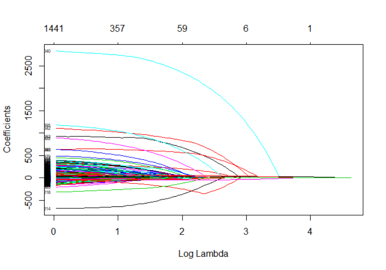
83
Figure 4.2: Number of features selected by the LASSO model as function of the Lambda
parameter
As anticipated, low values of lambda allow more variables in the model than high
values. Recall that a value of lambda that equals zero corresponds to the OLS with all the
explanatory variables in the model since there is no penalty on them.
Figure 4.3 illustrates the mean estimates of the MSE as a function of the lambda
parameter. The upper and lower standard deviations (error bar) of each mean estimate are
also illustrated. At the top of the graph, we have the number of features selected in the
model. The two vertical black dotted lines indicate the two selected lambda values (the
minimum value and the one-standard-error value) obtained via cross-validation. The un-
regularized model performs well with approximately 1360 variables. This corresponds to
the minimum value of lambda of 1.083. The unregularized model is the model that corre-

84
sponds to the minimum value of lambda that gives the minimum mean cross-validated
error. However, the most regularized model, with the optimal variance-bias trade-off, is
achieved with a lambda value of 3.158. This value is associated with the model with an
error within one standard error of the minimum error and select 257 features.
Figure 4.3: Cross-validated mean estimates of the MSE as a function of the Lambda pa-
rameter
4.4.3. Pricing value of the features.
Among the 9917 variables, the LASSO regression selects 257 features that have a
predictive power in explaining room price on Airbnb in San Francisco. Figure 4.4 pre-
sents the 15 most important significant positive and negative variables with their esti-
mates. The figure shows that the LASSO regression produces estimates that are con-
sistent with the hedonic price literature. Location affects rental price since the price in
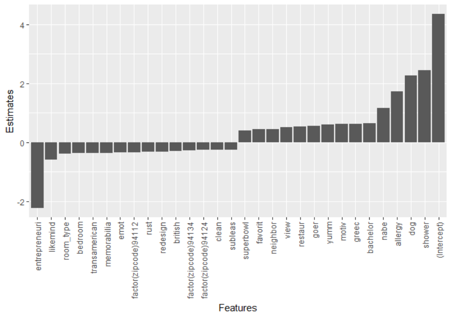
85
certain areas (zip codes 94112 and 94134, for example) are significantly lower compared
to other areas. Private rooms are also priced lower compared to entire homes or apart-
ments (the base variable for room type).
Figure 4.4: Estimates of the most important significant positive and negative variables
Tokens such as “redesign”, “rust”, and “subleas” are associated with lower rental
prices, implying these tokens have a negative effect on price. These tokens suggest, re-
spectively, that the rental unit has been redesigned, is rustier, and is being subleased. All
these suggestions can be associated with poor quality or at best an improvement or reno-
vation of the rental unit. An association with poor quality explains the negative estimates.
These tokens might capture unobserved time-unvarying characteristics of the rental (con-
struction materials, for example). An improvement or renovation of the rental unit by the
86
owner still suggests an initial poor quality of the rental unit and might imply that the to-
kens are related to time-varying attributes of the rental unit. These time-varying and time-
unvarying attributes are unobservable by the econometrician but are known by the host.
Information in the description section on the Airbnb platform can be used to approximate
the features that might be omitted in the hedonic model. This explains the reduction in
price errors observed when including, through the unigrams, information that might be
omitted in regression models.
A similar analysis can be conducted for the tokens with positive estimates. To-
kens such as “restaur”, “view”, “dog” “neighbor”, associated with higher rental prices,
imply that these tokens have a positive impact on the price. “restaur” and “neighbor”
suggest attributes such as the presence of restaurants or a good neighborhood which are
related to the location of the rental unit. The positive coefficient of a token such as “dog”
might be related to hosts allowing the presence of dogs in the premises. When features
related to the location (restaurant, and neighborhood) are commonly included in hedonic
models, those related to dogs are rarely accounted for. The use of textual analysis offers
the advantage to circumvent the pricing error that might be introduced by not including
such features. However, the use of tokens in the LASSO regression presents a limit: the
interpretability of the tokens. Not all the tokens have an intuitive interpretation, and the
interpretation is also subjective to the researcher. Methodologies that improve the textual
analysis to derive interpretable tokens will significantly increase its use in econometric
models.
87
4.5. Conclusion
This paper examines the effect of including features in the description of rooms
rented through Airbnb on the pricing error in a hedonic model. Hedonic models have
been widely used in real estate research to help evaluate consumers’ valuation of non-
market goods and services. Developed by Rosen (1974), this model has experienced con-
siderable improvements both theoretically and methodologically regarding its economet-
ric estimation. The omitted variable bias problem is one of the econometric issues that
has received a lot of attention. There are many variables that are related to the property
quality but that are unobserved by the econometrician. Omitting these variables in the
regression models will create inaccurate estimates of the price.
Nowak and Smith (2017) address the omitted variable bias problem using textual
analysis in the real estate literature. This study is the first to examine the same issue in the
hospitality literature. Using data on Airbnb in San Francisco, we augment a well-
specified hedonic model with a unigram representation of the words used to describe the
rental unit on the online platform. We test the hypothesis that the characteristics of the
rental units on the online platforms do not account for all the features needed to estimate
the price of those units in a hedonic price model correctly. However, the owners of the
rental units have information about the quality that they share through the description of
those units on the platform. Including those descriptions in the hedonic price model can
reduce the pricing error.
We test this hypothesis with a textual analysis methodology and the LASSO re-
gression. The textual analysis helps to decompose the text in the description into the sin-
gle words that compose it. Including the resulting large number of words into a standard

88
OLS regression would be infeasible due to the rank condition. We rely on the LASSO
regression that performs simultaneously shrinkage and feature selection. Results of our
analysis show that the LASSO performs well compared to a well-specified panel regres-
sion with time and location fixed effects. Including a unigram representation of the words
found in the description of the rooms reduces pricing error by more than 34%. Examina-
tion of the features selected by the LASSO suggests that including the BOW in the he-
donic model might address the OVB problem by accounting for time-varying and time-
unvarying quality features. However, the combination of LASSO and textual analysis in
the hedonic model do not produce easily interpretable estimates. Due to the importance of
including the BOW in the hedonic model, its potential to address the OVB problem, and
the increasing availability of user-generated contents online, future studies should ad-
vance the methodology needed to produce interpretable estimates generated by the com-
bination of textual analysis and hedonic price models.
89
CHAPTER 5 : GENERAL CONCLUSION
Machine learning and big data are intertwined concepts that refer fundamentally
to the same area of study. These concepts have gained in popularity in the recent years
thanks to the growth of the internet. Nowadays, consumers have access to a large assort-
ment of smart objects that collect a variety of data (sensory, location, behavior, texts, au-
dio, videos, etc.). These data, also referred to as big data, can be structured or unstruc-
tured and are generated in near real-time thus their important volume which gives them
the “big” attribute. Dealing with these big data require high-performance analytics and
machine learning is the branch of computer science that uses statistics to examine hiding
patterns in these big data. The use of big data and machine learning have found their ap-
plication in industries such as healthcare, transportation, online retail, government, travel,
and hospitality. Can the success observed in these industries be replicated in economics?
The present dissertation examines this question with three essays on the application of
machine learning in economics.
The first essay uses sentiment analysis to derive the sentiments hidden in the re-
views left by customers on the Airbnb in Boston. Using the sentiment as a measure of
quality, it explores the relationship between the reviews and the price set by guests on the
online platform. The results of the hedonic spatial autoregressive model applied to rental
room prices on Airbnb in the study area show that prices are influenced not only by the
characteristics of the room, and the features of the neighborhood, but also by the reviews
left by hosts. The second essay predicts consumer preferences by mining beer reviews
posted by enthusiasts on an online platform. It uses a text categorization approach to dis-
cuss the predictive capability of the words used in the reviews by customers to express
90
their preferences. Relying on the random forest algorithm, this essay shows that the
words used in the reviews can help predict consumers’ preferences and the words which
occur in multiple reviews do not effectively categorize the reviews than the less frequent
terms. The essay also identifies from the reviews the beer attributes, such as those related
to the smell or taste, look, and overall quality of the beer, as the most important features
in predicting consumers’ preferences. The third and last essay addresses an issue that af-
fects the reliability of estimates in hedonic price models: the omitted variable bias. It
shows that by using the words in the description of the rental properties in the estimation
procedures of the model, we can reduce significantly the bias created by omitted varia-
bles. The description can account for variables that are not readily measurable but that are
important in getting reliable estimates in the hedonic model. This essay also emphases a
limitation of certain machine learning methods: the difficulty in interpreting some results
derived from the models. The interpretation of certain variables of the LASSO regression
model can be subjective to the econometrician.
Big data and machine learning can advance economics in various ways. They can
make available large volume of data that represents the real behavior of economic agents
in non-hypothetical situations. They can advance applied research in economics by ad-
dressing some limitations such as the omitted variable bias encountered in econometrics.
However, the effective use of big data will also require the training of the next generation
of economists in the techniques, tools, and skills needed to derive value from it. To en-
courage the adoption of machine learning methods in economics, it is also necessary to
encourage scholarly activities on the development or adaptation of existing machine
learning methodologies to causal inference studies.
91
GLOSSARY
Accuracy: The number of correct predictions from all the predictions made by a machine
learning algorithm.
Area under the curve (AUC): Likelihood that a classifier will rank a randomly drawn
positive higher than a uniformly drawn random negative.
Bag of words (BOW): Model of representation of text data used in natural language pro-
cessing and which consists on extracting words from a raw text and recording their occur-
rence in the text.
Cross validation: Resampling method to evaluate predictive models that consists on
running the model on different subsets of the data
Decision tree: Machine learning method that map the possible outcomes against one an-
other based on values that minimizes a loss function. The result is a tree-like decision
rule.
False negatives: Proportion of positive outcomes wrongly predicted as negative out-
comes
False positives: Proportion of negative outcomes wrongly predicted as positives out-
comes
K nearest neighbors (KNN): Approach that predicts the class of an object using its K-
closest neighbors. Closeness is based on a distance defined by the user. Euclidian dis-
tance is the most commonly used distance metric.
Kappa statistic: Metric used to evaluate the performance of a classifier by comparing the
accuracy achieved by the classifier with its expected accuracy (random chance).
Linear discriminant analysis (LDA): Classification method that uses a mathematical
path to predict the probability of an object to belong to a group based on the predictor
characteristics
92
Machine learning: Branch of artificial intelligence that uses computational methods to
learn from data, identify patterns, and make decisions. Machine learning methods are
generally categorized into supervised and unsupervised learning algorithms. Supervised
learning algorithms use know input and output data to train a model that best approxi-
mates the relationship between them so that it will predict future outputs. Unsupervised
learning algorithms task consists of finding hidden patterns or the underlying structure
present in a set of input data. As part of machine learning algorithms are also Semi-
supervised learning which borrows from supervised and unsupervised technics and rein-
forcement learning algorithms which learn through trials and errors which actions attain a
complex objective or goal.
Natural language processing (NLP): Field of artificial intelligence that deals with help-
ing computers understand, interpret, and manipulate human language text or speech.
N-gram: set of contiguous sequence of n words in a text data. Unigram, bigram, and tri-
gram correspond to a decomposition of the text into the single words, pairs or words, or
sequence of three words.
Random forest: machine learning method for classification and regression that uses an
ensemble of decision trees
Sentiment analysis: Area of Natural Language Processing that consists on identifying
and extracting subjective sentiments or opinions from textual contents.
Stemming: In natural language processing, the task of reducing a word (inflected or deri-
vationally related) to its root or base also called stem.
Support vector machines (SVMs): Ordinary Least Squares (OLS) regressions estimates
parameters that minimize the sum of squared of residuals (SSR). These estimates are sen-
sitive to the presence of outliers. However, minimization metric such as the Huber func-
tion performs better than the SSR when the data contains influential observations. The
Huber function uses the absolute residuals for residuals whose values are large but uses
the squared residuals when the values of the residuals are small. SVMs minimize the ef-
fects of the residuals using the Huber function and within a threshold ε defined by the
93
user. Only data points with absolute difference greater than the threshold contributes to
the regression fit. This approach ensures that large outliers have less influence on the re-
gression (since the squared residuals are not used).
Text categorization: Automatic assignment or classification of texts into predefined cat-
egories.
Tokenization: In natural Language processing, the tokenization is the task of decompos-
ing text data into the pieces of words or terms, also called tokens, composing the text.
True negatives: proportion of negative outcomes correctly predicted by a machine learn-
ing algorithm
True positives: proportion of positive outcomes correctly predicted by a machine learn-
ing algorithm
94
REFERENCES
Abbott, J.K., and H.A. Klaiber. 2011. "An embarrassment of riches: Confronting omitted
variable bias and multi-scale capitalization in hedonic price models." Review of
Economics and Statistics 93:1331-1342.
Anselin, L. 1988. "Lagrange multiplier test diagnostics for spatial dependence and spatial
heterogeneity." Geographical Analysis 20:1-17.
Anselin, L., and A.K. Bera. 1998. "Spatial dependence in linear regression models with
an introduction to spatial econometrics." Statistics Textbooks and Monographs
155:237-290.
Archak, N., A. Ghose, and P.G. Ipeirotis. 2011. "Deriving the pricing power of product
features by mining consumer reviews." Management Science 57:1485-1509.
Balinsky, A.A., H.Y. Balinsky, and S.J. Simske (2010) "On helmholtz's principle for
documents processing." In Proceedings of the 10th ACM symposium on
Document engineering. ACM, pp. 283-286.
Bates, D., et al. 2015. "Fitting Linear Mixed-Effects Models Usinglme4." Journal of
Statistical Software 67.
Bautin, M., L. Vijayarenu, and S. Skiena (2008) "International Sentiment Analysis for
News and Blogs." In ICWSM.
Bayer, P., F. Ferreira, and R. McMillan. 2007. "A unified framework for measuring
preferences for schools and neighborhoods." Journal of political economy
115:588-638.
Bayer, P., N. Keohane, and C. Timmins. 2009. "Migration and hedonic valuation: The
case of air quality." Journal of environmental economics and management 58:1-
14.
95
Bespalov, D., et al. (2011) "Sentiment classification based on supervised latent n-gram
analysis." In Proceedings of the 20th ACM international conference on
Information and knowledge management. ACM, pp. 375-382.
Biber, D. 1991. Variation across speech and writing: Cambridge University Press.
Bivand, R., J. Hauke, and T. Kossowski. 2013. "Computing the Jacobian in Gaussian
spatial autoregressive models: an illustrated comparison of available methods."
Geographical Analysis 45:150-179.
Bivand, R., and G. Piras (2015) "Comparing implementations of estimation methods for
spatial econometrics." In., American Statistical Association.
Blal, I., and M.C. Sturman. 2014. "The Differential Effects of the Quality and Quantity of
Online Reviews on Hotel Room Sales." Cornell Hospitality Quarterly 55:365-
375.
Breiman, L. 1996. "Bagging predictors." Machine Learning 24:123-140.
---. 2017. Classification and regression trees: Routledge.
---. 2001. "Random Forests." Machine Learning 45:5-32.
Brooks, R.C. 1957. "" Word-of-Mouth" Advertising in Selling New Products." The
Journal of Marketing:154-161.
Cavnar, W.B., and J.M. Trenkle. 1994. "N-gram-based text categorization." Ann Arbor
MI 48113:161-175.
Chay, K.Y., and M. Greenstone. "Does air quality matter? Evidence from the housing
market." National Bureau of Economic Research.
---. 2005. "Does air quality matter? Evidence from the housing market." Journal of
political economy 113:376-424.
96
Chen, P.-Y., S. Dhanasobhon, and M.D. Smith. 2008. "All reviews are not created equal:
The disaggregate impact of reviews and reviewers at amazon. com."
Chevalier, J.A., and D. Mayzlin. 2006. "The effect of word of mouth on sales: Online
book reviews." Journal of Marketing Research 43:345-354.
Chu, C., et al. 2012. "Does feature selection improve classification accuracy? Impact of
sample size and feature selection on classification using anatomical magnetic
resonance images." Neuroimage 60:59-70.
Cirer Costa, J.C. 2013. "Price formation and market segmentation in seaside
accommodations." International Journal of Hospitality Management 33:446-455.
Cohen, J. 1960. "A coefficient of agreement for nominal scales." Educational and
psychological measurement 20:37-46.
Cropper, M.L., L.B. Deck, and K.E. McConnell. 1988. "On the choice of funtional form
for hedonic price functions." The Review of Economics and Statistics:668-675.
Cui, H., V. Mittal, and M. Datar (2006) "Comparative experiments on sentiment
classification for online product reviews." In AAAI. pp. 1265-1270.
d'Aspremont, C., J.J. Gabszewicz, and J.-F. Thisse. 1979. "On Hotelling's" Stability in
competition"." Econometrica: journal of the Econometric Society:1145-1150.
Davlasheridze, M., K. Fisher-Vanden, and H. Allen Klaiber. 2017. "The effects of
adaptation measures on hurricane induced property losses: Which FEMA
investments have the highest returns?" Journal of environmental economics and
management 81:93-114.
de Oliveira Santos, G.E. 2016. "Worldwide hedonic prices of subjective characteristics of
hostels." Tourism Management 52:451-454.
De Vany, A., and W.D. Walls. 1999. "Uncertainty in the movie industry: Does star power
reduce the terror of the box office?" Journal of cultural economics 23:285-318.
97
De Vries, A.P., and T. Roelleke (2005) "Relevance information: a loss of entropy but a
gain for IDF?" In Proceedings of the 28th annual international ACM SIGIR
conference on Research and development in information retrieval. ACM, pp. 282-
289.
Dellarocas, C., X. Zhang, and N.F. Awad. 2007. "Exploring the value of online product
reviews in forecasting sales: The case of motion pictures." Journal of Interactive
Marketing 21:23-45.
Dietterich, T.G. 2000. "An Experimental Comparison of Three Methods for Constructing
Ensembles of Decision Trees: Bagging, Boosting, and Randomization." Machine
Learning 40:139-157.
Domingos, P., and G. Hulten (2000) "Mining high-speed data streams." In Proceedings
of the sixth ACM SIGKDD international conference on Knowledge discovery and
data mining. ACM, pp. 71-80.
Eisenmann, T., G. Parker, and M.W. Van Alstyne. 2006. "Strategies for two-sided
markets." Harvard business review 84:92.
Espinet, J.M., et al. 2003. "Effect on prices of the attributes of holiday hotels: a hedonic
prices approach." Tourism Economics 9:165-177.
Feinerer, I., et al. 2013. "The textcat package for n-gram based text categorization in R."
Journal of Statistical Software 52:1-17.
Finn, A., N. Kushmerick, and B. Smyth (2002) "Genre classification and domain transfer
for information filtering." In European Conference on Information Retrieval.
Springer, pp. 353-362.
Floyd, K., et al. 2014. "How Online Product Reviews Affect Retail Sales: A Meta-
analysis." Journal of Retailing 90:217-232.
Fonti, V., and E. Belitser (2017) "Feature Selection using LASSO." In.
98
Gabszewicz, J.J., and J.-F. Thisse. 1979. "Price competition, quality and income
disparities." Journal of economic theory 20:340-359.
Goodwin, K., B. Waller, and H.S. Weeks. 2014. "The impact of broker vernacular in
residential real estate." Journal of Housing Research 23:143-161.
Gravelle, H., R. Santos, and L. Siciliani. 2014. "Does a hospital's quality depend on the
quality of other hospitals? A spatial econometrics approach." Reg Sci Urban Econ
49:203-216.
Green, R., and P.H. Hendershott. 1996. "Age, housing demand, and real house prices."
Regional Science and Urban Economics 26:465-480.
Greiff, W.R. (1998) "A theory of term weighting based on exploratory data analysis." In
Proceedings of the 21st annual international ACM SIGIR conference on Research
and development in information retrieval. ACM, pp. 11-19.
Gretzel, U., and K.H. Yoo (2008) "Use and Impact of Online Travel Reviews." In P.
O’Connor,W. Höpken, and U. Gretzel eds. Information and Communication
Technologies in Tourism 2008: Proceedings of the International Conference in
Innsbruck, Austria, 2008. Vienna, Springer Vienna, pp. 35-46.
Grislain-Letrémy, C., and A. Katossky. 2014. "The impact of hazardous industrial
facilities on housing prices: A comparison of parametric and semiparametric
hedonic price models." Regional Science and Urban Economics 49:93-107.
Haag, J., R. Rutherford, and T. Thomson. 2000. "Real Estate Agent Remarks: Help or
Hype?" Journal of Real Estate Research 20:205-215.
Hagenau, M., M. Liebmann, and D. Neumann. 2013. "Automated news reading: Stock
price prediction based on financial news using context-capturing features."
Decision Support Systems 55:685-697.
Hagiu, A., and J. Wright. 2015. "Multi-sided platforms." International Journal of
Industrial Organization 43:162-174.
99
Hamermesh, D.S. 2013. "Six Decades of Top Economics Publishing: Who and How?"
Journal of Economic Literature 51:162-172.
Han, E.-H.S., G. Karypis, and V. Kumar (2001) "Text categorization using weight
adjusted k-nearest neighbor classification." In Pacific-asia conference on
knowledge discovery and data mining. Springer, pp. 53-65.
Harrison, D., and D.L. Rubinfeld. 1978. "Hedonic housing prices and the demand for
clean air." Journal of environmental economics and management 5:81-102.
Hoerl, A.E., and R.W. Kennard. 1970. "Ridge regression: Biased estimation for
nonorthogonal problems." Technometrics 12:55-67.
Hotelling, H. 1929. "Stability in competition." The economic journal 39:41-57.
Hu, M., and B. Liu (2004) "Mining and summarizing customer reviews." In Proceedings
of the tenth ACM SIGKDD international conference on Knowledge discovery and
data mining. ACM, pp. 168-177.
Hu, N., L. Liu, and J.J. Zhang. 2008. "Do online reviews affect product sales? The role of
reviewer characteristics and temporal effects." Information Technology and
Management 9:201-214.
Kim, Y., and J. Srivastava (2007) "Impact of social influence in e-commerce decision
making." In Proceedings of the ninth international conference on Electronic
commerce. ACM, pp. 293-302.
Klein, L.R. 1998. "Evaluating the potential of interactive media through a new lens:
Search versus experience goods." Journal of Business Research 41:195-203.
Kozinets, R.V., et al. 2010. "Networked narratives: Understanding word-of-mouth
marketing in online communities." Journal of marketing 74:71-89.
Kuhn, M., and K. Johnson. 2013. Applied predictive modeling: Springer.
100
Kuminoff, N.V., C.F. Parmeter, and J.C. Pope. 2010. "Which hedonic models can we
trust to recover the marginal willingness to pay for environmental amenities?"
Journal of environmental economics and management 60:145-160.
Kursa, M.B., and W.R. Rudnicki. 2010. "Feature selection with the Boruta package." J
Stat Softw 36:1-13.
Larson, R.R. (2010) "Introduction to information retrieval." In., Wiley Online Library.
Le Gallo, J., C. Ertur, and C. Baumont. 2003. "A Spatial Econometric Analysis of
Convergence Across European Regions, 1980–1995."99-129.
Lesage, J.P. 2008. "An Introduction to Spatial Econometrics." Revue d'économie
industrielle 123:19-44.
Lewis, D.D., et al. 2004. "Rcv1: A new benchmark collection for text categorization
research." Journal of Machine Learning Research 5:361-397.
Li, X., and L.M. Hitt. 2010. "Price effects in online product reviews: An analytical model
and empirical analysis." MIS quarterly:809-831.
Litvin, S.W., R.E. Goldsmith, and B. Pan. 2008. "Electronic word-of-mouth in hospitality
and tourism management." Tourism Management 29:458-468.
Liu, B., M. Hu, and J. Cheng (2005) "Opinion observer: analyzing and comparing
opinions on the web." In Proceedings of the 14th international conference on
World Wide Web. ACM, pp. 342-351.
Liu, Y. 2006. "Word of mouth for movies: Its dynamics and impact on box office
revenue." Journal of marketing 70:74-89.
Luca, M. 2016. "Reviews, reputation, and revenue: The case of Yelp. com."
Mauri, A.G., and R. Minazzi. 2013. "Web reviews influence on expectations and
purchasing intentions of hotel potential customers." International Journal of
Hospitality Management 34:99-107.
101
Menze, B.H., et al. 2009. "A comparison of random forest and its Gini importance with
standard chemometric methods for the feature selection and classification of
spectral data." BMC Bioinformatics 10:213.
Metzler, D. (2008) "Generalized inverse document frequency." In Proceedings of the
17th ACM conference on Information and knowledge management. ACM, pp.
399-408.
Meyer, D., K. Hornik, and I. Feinerer. 2008. "Text mining infrastructure in R." Journal of
Statistical Software 25:1-54.
Mobley, L.R. 2003. "Estimating hospital market pricing: an equilibrium approach using
spatial econometrics." Regional Science and Urban Economics 33:489-516.
Mobley, L.R., H.E. Frech, and L. Anselin. 2009. "Spatial Interaction, Spatial Multipliers
and Hospital Competition." International Journal of the Economics of Business
16:1-17.
Motta, M. 1993. "Endogenous quality choice: price vs. quantity competition." The
Journal of Industrial Economics:113-131.
Murray, J.M., C.M. Delahunty, and I.A. Baxter. 2001. "Descriptive sensory analysis:
past, present and future." Food Research International 34:461-471.
Mussa, M., and S. Rosen. 1978. "Monopoly and product quality." Journal of economic
theory 18:301-317.
Nazir, N.N.M., N. Othman, and A.H. Nawawi. 2015. "Role of Green Infrastructure in
Determining House Value in Labuan Using Hedonic Pricing Model." Procedia -
Social and Behavioral Sciences 170:484-493.
Nicolau, J.L., and R. Sellers. 2010. "The quality of quality awards: Diminishing
information asymmetries in a hotel chain." Journal of Business Research 63:832-
839.
102
Nielsen, F.Å. 2011. "A new ANEW: Evaluation of a word list for sentiment analysis in
microblogs." arXiv preprint arXiv:1103.2903.
Nilsson, R., et al. 2007. "Consistent feature selection for pattern recognition in
polynomial time." Journal of Machine Learning Research 8:589-612.
Nowak, A., and P. Smith. 2017. "Textual analysis in real estate." Journal of Applied
Econometrics 32:896-918.
O’Connor, P. 2008. "User-generated content and travel: A case study on Tripadvisor.
com." Information and communication technologies in tourism 2008:47-58.
Ogden, M. 2001. "Marketing truth: hearing is believing." The Business Journal 16:17.
Öğüt, H., and B.K. Onur Taş. 2012. "The influence of internet customer reviews on the
online sales and prices in hotel industry." The Service Industries Journal 32:197-
214.
Palmquist, R.B. 2005. "Property value models." Handbook of environmental economics
2:763-819.
Pang, B., and L. Lee. 2008. "Opinion mining and sentiment analysis." Foundations and
Trends® in Information Retrieval 2:1-135.
Pang, B., L. Lee, and S. Vaithyanathan (2002) "Thumbs up?: sentiment classification
using machine learning techniques." In Proceedings of the ACL-02 conference on
Empirical methods in natural language processing-Volume 10. Association for
Computational Linguistics, pp. 79-86.
Pavlou, P.A., and A. Dimoka. 2006. "The nature and role of feedback text comments in
online marketplaces: Implications for trust building, price premiums, and seller
differentiation." Information Systems Research 17:392-414.
Popescu, A.-M., and O. Etzioni (2007) "Extracting product features and opinions from
reviews." In Natural language processing and text mining. Springer, pp. 9-28.
103
Rosen, S. 1974. "Hedonic prices and implicit markets: product differentiation in pure
competition." Journal of political economy 82:34-55.
Sander, H., S. Polasky, and R.G. Haight. 2010. "The value of urban tree cover: A hedonic
property price model in Ramsey and Dakota Counties, Minnesota, USA."
Ecological Economics 69:1646-1656.
Sarvabhotla, K., P. Pingali, and V. Varma. 2010. "Supervised learning approaches for
rating customer reviews." Journal of Intelligent Systems 19:79-94.
Sati, Z.E. 2017. "Evaluation of Big Data and Innovation Interaction in Increase Supply
Chain Competencies." Üniversitepark Bülten| Universitepark Bulletin.
Schumaker, R.P., and H. Chen. 2009. "A quantitative stock prediction system based on
financial news." Information Processing & Management 45:571-583.
---. 2009. "Textual analysis of stock market prediction using breaking financial news."
ACM Transactions on Information Systems 27:1-19.
Senecal, S., and J. Nantel. 2004. "The influence of online product recommendations on
consumers’ online choices." Journal of Retailing 80:159-169.
Seo, K., A. Golub, and M. Kuby. 2014. "Combined impacts of highways and light rail
transit on residential property values: a spatial hedonic price model for Phoenix,
Arizona." Journal of Transport Geography 41:53-62.
Shaked, A., and J. Sutton. 1983. "Natural oligopolies." Econometrica: journal of the
Econometric Society:1469-1483.
Shannon, C. 1948. "(1948)," A Mathematical Theory of Communication", Bell System
Technical Journal, vol. 27, pp. 379-423 & 623-656, July & October."
Sparck Jones, K. 1972. "A statistical interpretation of term specificity and its application
in retrieval." Journal of documentation 28:11-21.
104
Sparks, B.A., and V. Browning. 2011. "The impact of online reviews on hotel booking
intentions and perception of trust." Tourism Management 32:1310-1323.
Stefanowicz, P. 2013. "Sensory evaluation of food principles and practices." Journal of
Wine Research 24:80-80.
Tibshirani, R. 1996. "Regression shrinkage and selection via the lasso." Journal of the
Royal Statistical Society. Series B (Methodological):267-288.
Varela, P., and G. Ares. 2012. "Sensory profiling, the blurred line between sensory and
consumer science. A review of novel methods for product characterization." Food
Research International 48:893-908.
Vermeulen, I.E., and D. Seegers. 2009. "Tried and tested: The impact of online hotel
reviews on consumer consideration." Tourism Management 30:123-127.
Viglia, G., R. Minazzi, and D. Buhalis. 2016. "The influence of e-word-of-mouth on
hotel occupancy rate." International Journal of Contemporary Hospitality
Management 28:2035-2051.
Wauthy, X. 1996. "Quality choice in models of vertical differentiation." The Journal of
Industrial Economics:345-353.
Ye, Q., R. Law, and B. Gu. 2009. "The impact of online user reviews on hotel room
sales." International Journal of Hospitality Management 28:180-182.
Ye, Q., et al. 2011. "The influence of user-generated content on traveler behavior: An
empirical investigation on the effects of e-word-of-mouth to hotel online
bookings." Computers in Human Behavior 27:634-639.
Ye, Q., Z. Zhang, and R. Law. 2009. "Sentiment classification of online reviews to travel
destinations by supervised machine learning approaches." Expert Systems with
Applications 36:6527-6535.
105
Yu, J., et al. (2011) "Aspect ranking: identifying important product aspects from online
consumer reviews." In Proceedings of the 49th Annual Meeting of the
Association for Computational Linguistics: Human Language Technologies-
Volume 1. Association for Computational Linguistics, pp. 1496-1505.
Yu, X., et al. 2012. "Mining Online Reviews for Predicting Sales Performance: A Case
Study in the Movie Domain." IEEE Transactions on Knowledge and Data
Engineering 24:720-734.
Zhang, L., et al. 2013. "The impact of online user reviews on cameras sales." European
Journal of Marketing 47:1115-1128.
Zhang, L., B. Ma, and D.K. Cartwright. 2013. "The impact of online user reviews on
cameras sales." European Journal of Marketing 47:1115-1128.
Zhang, M.-L., and Z.-H. Zhou. 2006. "Multilabel neural networks with applications to
functional genomics and text categorization." IEEE Transactions on Knowledge
and Data Engineering 18:1338-1351.
Zhang, Z., Q. Ye, and R. Law. 2011. "Determinants of hotel room price: An exploration
of travelers' hierarchy of accommodation needs." International Journal of
Contemporary Hospitality Management 23:972-981.
Zhang, Z., et al. 2010. "The impact of e-word-of-mouth on the online popularity of
restaurants: A comparison of consumer reviews and editor reviews." International
Journal of Hospitality Management 29:694-700.

106
VITA
ABDELAZIZ LAWANI
EDUCATION
North Carolina State University
M.A., Economics
2013
Abomey-Calavi University (Benin)
M.Sc. Agricultural and Development Economics, and Rural Sociology
2008
Abomey-Calavi University (Benin)
B.Sc. Agronomy
2007
WORKING PAPERS
Lawani, A., M. Reed., M. Tyler., Zheng Y. 2017. “Impact of online reviews on price: Evi-
dence from sentiment analysis of Airbnb reviews in Boston.”
Lawani, A. 2017. “Beer quality and preferences: sensory analysis of reviews scrapped from
beeradvocates.com.”
Lawani, A. 2017. “Return and volatility transmission on the cryptocurrency market.”
Lawani, A., M. Reed., R. Fiamohe. 2016. “Impact of Food Reserve Programs on Price Levels
and Volatility: Natural Experiment from Benin Cereals Markets in West Africa.”
Lawani, A., S. Saghaian, Yuqing Zheng. 2015. Tourism Demand Analysis in the US: An Al-
most Ideal Demand System Approach.
GRANTS, AWARDS, FELLOWSHIPS & HONORS
ACP-EU Technical Centre for Agricultural and Rural Co-operation (CTA) grant
(€19998)
2018
Clinton Foundation Honor Roll (CGI U) 2017
Future Leaders Forum of the Association for International Agriculture and Rural
Development scholarship
2017
University of Kentucky Sustainability Grant ($6000) 2017
Technical Centre for Agricultural and Rural Co-operation grant for the project
“ICT4Ag” (€7800)
2017
AWF Species Protection Grant ($20,000) with the Laboratory of Applied ecology
(Benin)
2016
Finalist AAEA Extension Competition 2016
University of Kentucky Research Activity Award (2016-2017) ($3000) 2016
University of Kentucky travel grant ($400) 2016
Clinton Global Initiative Grant (multiple grants for project implementation and trav-
2016

107
el)
U.S. Embassy in Benin Public Affairs Grants ($2000) 2016
University of Kentucky Sustainability Grant ($4600) 2015
Norman E. Borlaug Leadership Enhancement in Agriculture Program Grant
($20,000)
2015
IDEA WILD Grant ($800) 2015
Alumni Engagement Innovation Fund for the project Youth and Gender-Based Vio-
lence, United States Department ($17,000)
2014
Alumni Engagement Innovation Fund for the project Youth Entrepreneurs Partners
(YEP), United, States Department ($25,000)
2013
Graduate Student Research and Teaching Assistantship at University of Kentucky
2013 -
18
Graduate Student Assistantship at North Carolina State University 2012
Fulbright scholarship 2010
Travel Grant by the African Technology Policy Studies Network (ATPS) 2011
African Technology Policy Studies Network (ATPS) Research Award ($10,000) 2010
Travel Grant by DIVESITAS for the OSC2- Cape Town, South Africa 2010
Excellence Scholarship from Benin Government for Undergraduate Studies in
Agronomy and Graduate Studies in Agricultural Economics at Abomey-Calavi Uni-
versity, Benin
2002-
07
CONFERENCES
Southern Agricultural Economics Association (SAEA) Annual Meeting
2018
Information and Communications Technology for Development 10
th
Conference
(Lusaka, Zambia)
2018
AERE at the 87
th
Southern Economic Association Annual Conference, Tampa,
Florida
2017
Western Economic Association International (WEAI), 92
nd
Annual Conference -
San Diego, California
2017
Association for International Agriculture and Rural Development (AIARD) Annu-
al meeting
2017
Southern Agricultural Economics Association (SAEA) Annual Meeting - Presenter
and Session Chair, Mobile Alabama
2017
Agricultural and Applied Economics Association, Annual Meeting, Boston 2016

108
Clinton Global Initiatives Annual Meeting, New York 2016
Clinton Global Initiatives University, University of California Berkley 2016
World Food Prize, Des Moines, Iowa 2015
2015 Concordia Summit, New York. 2015
19th Annual Conference of the Yale Chapter of the International Society of Tropi-
cal Foresters, New Haven, CT
2013
2012 ATPS Annual Conference on “Emerging Paradigms, Technologies and In-
novations for Sustainable Development: Global Imperatives and African Reali-
ties”, Addis Ababa, Ethiopia
2012
2011 ATPS Annual Conference on “Strengthening Linkages between Policy Re-
search and Policymaking for African Development,” Mombasa, Kenya
2011
2010 ATPS Annual Conference on “The state of science, technology and innova-
tion in Africa: Implications for Achieving the Millennium Development Goals,”
Cairo, Egypt
2010
ATPS Annual Conference on “Africa’s response to global challenges through sci-
ence technology and innovation,” Abuja, Nigeria.
2009
DIVESITAS OSC2- Biodiversity and society: understanding connections, adapting
to change, Cape Town, South Africa
2009
Abomey-Calavi University Conference on “Sciences, Cultures and Technologies,”
Benin.
2009
Conference on chronic poverty, CPRC, Cotonou, Benin. 2007
14th Annual Conference of the Beninese Association for pastoralism (ABePa), Co-
tonou, Benin.
2007
P
ROFESSIONAL & RESEARCH EXPERIENCES
Lecturer at the University of Kentucky
2015-2016
Lecturer at the Faculty of Economics and Management of the University
of Abomey-Calavi
2015
Technical assistant and data Analyst at CEBEDES-Benin
2009 - 2010
Technical Assistant, CEBEDES-Benin
2008 - 2009
